Measurements
A measurement is a certain observable of your experiment, it may be a real measureable quantity or a (comlex or real) non-measureable quantity of an experiment. This can be, for example, a Moessbauer spectrum, a thin film reflectivity, the photon field intensity inside a sample, the complex energy-dependent scattering amplitude, and so on.
All measurement types are a Measurement object.
Only those that calculate real and observable quantities are of type FitMeasurement, which means that those measurements can be fit to a data set.
These two classes are base classes which means you do not have to deal with them directly, they are used for internal purposes of Nexus only.
However, in case you are not sure whether you can fit a measurement or not have a look to the API Reference of the specific measurement.
You can see a base class in the constructor documentation.
Only if it is nexus.clib.cnexus.FitMeasurement the measurement is taken by the Fit module.
You can pass any Measurement object to the Optimizer module.
Measurement types
Nexus provides a couple of different measurement types. The following lists show fittable and non-fittable measurements implemented at the moment. Electronic and nuclear scattering refer to pure prompt scattering at electrons and delayed scattering due to nuclear interactions, respectively. For some methods you can specify which scattering contributions are taken into account.
Non-fittable measurements
Methods with pure electronic contributions:
Amplitudes: Calculates the complex electronic scattering amplitudes after each object in the experiment.Matrices: Calculates the complex electronic scattering matrices after each object in the experiment.JonesVectors: Calculates the complex electronic Jones vector after each object in the experiment.Intensities: Calculates the electronic scattering intensities after each object in the experiment.FieldAmplitude: Calculates the complex electronic field amplitude inside a sample.FieldIntensity: Calculates the absolute electronic field intensity inside a sample.ReflectivityAmplitude: Calculates the angular-dependent complex electronic amplitude of the experiment with a sample in reflection geometry whose incidence angle is changed.TransmissionAmplitude: Calculates the angular-dependent complex electronic amplitude of the experiment with a sample in transmission geometry whose incidence angle is changed.
Methods with electronic and nuclear scattering:
AmplitudeSpectrum: Calculates the complex energy-dependent Jones vector of the experiment.AmplitudeTime: Calculates the complex time-dependent Jones vector of the experiment.EnergyTimeAmplitude: Calculates the detuning and time-dependent complex Jones vector of an experiment where one sample is energy-detuned (Doppler-detuned) with respect to all others.
Amplitude methods are of Measurement type, return complex quantities, cannot be fit to experimental data, and are intended for theoretical calculations.
Intensities and FieldIntensity return real quantities but cannot be fit.
Thickness or angular distributions cannot be applied to non-fittable measurements because they assume incoherent addition of intensities.
Fittable measurements
Methods with pure electronic contributions:
Reflectivity: Calculates the electronic intensity of an experiment with a sample in reflection geometry with the incidence angle being scanned.Transmission: Calculates the electronic intensity of an experiment with a sample in (gracing-incidence) transmission geometry with the incidence angle being scanned.
Methods with electronic and nuclear scattering:
MoessbauerSpectrum: Calculates the velocity-dependent coherent intensity of an experiment.EmissionSpectrum: Calculates an velocity-dependent emission intensity of an experiment. See comments there for the exact model.EnergySpectrum: Calculates the detuning-dependent coherent transmission intensity of an experiment.TimeSpectrum: Calculates the time-dependent coherent transmission intensity of an experiment.EnergyTimeSpectrum: Calculates the detuning and time-dependent coherent intensity of an experiment where one sample is energy-detuned (Doppler-detuned) with respect to all others.IntegratedEnergyTimeSpectrum: Calculates the time-integrated coherent intensity of anEnergyTimeSpectrumobject.NuclearReflectivity: Calculates the pure nuclear delayed intensity of an experiment. One sample is in reflection geometry with the incidence angle being scanned.NuclearReflectivityEnergy: Calculates the energy-integrated intensity of an experiment. One sample is in reflection geometry with the incidence angle being scanned.
These methods are of FitMeasurement type, return real quantities and are intended to fit experimental data sets.
Parameters
Every Measurement needs at least an Experiment or a Sample, depending on the measurement type.
Here, all information on the experimental setup are given, needed by the measurement method.
The measurement is just a certain view onto the experiment and returns the calculated property.
A FitMeasurement always needs an Experiment.
If you want to fit a data set you also have to provide the measured data.
For a MoessbauerSpectrum, for example, you have to provide the measured velocity and intensity_data.
What is exactly needed depends on the Measurement type.
A lot of additional parameters influence a real measurement.
To account for experimental conditions, a FitMeasurment has a couple of additional parameters.
scaling: The scaling factor to scale the theoretical curve to the measured intensity. It can be a float,nx.Varorauto.
background: An intensity background added to the scaled theoretical curve. It can be a float,nx.Varorauto.
offset: An offset in the non-dependent variable to account for an experimental offset. Not available for Energy or Moessbauer spectra as it has the same influence as the isomer shift.New in version 1.1.0.
kernel_type(some methods): A Gaussian or Lorentzian kernel can be used to convolute the theoretical curve with the experimental resolution function. This is either the energy resolution of a Moessbauer source, the time resolution of an APD or the angular resolution of a reflectivity.
resolution: FWHM of the Gaussian or Lorentzian used in the resolution kernel.
distribution_points: In case thickness or angular distributions should be taken into account, specify a value larger than one. The thickness or angular distribution of each object is then approximated by the given number of points. Typically, if used, the value should be larger than 7.
fit_weight: Relative weight of the specific measurement in multi-measurement fits.
residual: The residual is used to weight the difference between the measured data and the theoretical curves properly. The standard residual depends on the measurement type you use, see residual.
The following parameters are Var objects and can be fit:
scaling
background
resolution
Measurement functor
A Measurement object is a functor.
It is quite similar to a function in the sense that it can be called but it can hold certain parameters and object states provided during initialization.
First, the object has to be initialized and after the initialization the calculation (function call) can be performed.
For example, a Moessbauer spectrum would be created and calculated like this
import nexus as nx
import numpy as np

# definitions for experiment would be here
# ....
# exp = nx.Experiment(....)

# define a range of the calculation
velocities = np.linspace(-10, 10, 2001)  # in mm/s

# define the Moessbauer spectrum object
spectrum = nx.MoessbauerSpectrum(experiment = exp,
                                 velocity = velocities)

# the spectrum functor is now initialized with the parameters experiment and velocity

# now the spectrum can be called as it would be a function
intensity = spectrum()
# or equivalently by the Calculate() method
intensity = spectrum.Calculate()
# which is a bit more intuitive because you know what the functor actually does.

print(intensity)
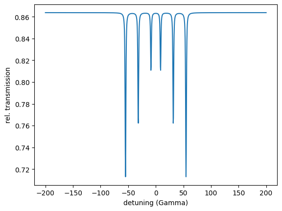
Energy Spectrum
The EnergySpectrum method is the most general class to calculate energy dependent experiments.
To calculate Moessbauer spectra or a conversion electron Moessbauer (CEM) spectra it is recommended to use the specific implementations, which just call this method with special initialization parameters.
You can specify the standard parameters for a FitMeasurement, see Measurements. Note, that the standard kernel type for convolutions in Nexus is Gaussian. The convolution of a Gaussian kernel and a Lorentzian resonance will result in a Voigt profile. Depending on your experiment this may not what you want to simulate, so you can choose a Lorentzian kernel as well.
The specific parameters for the EnergySpectrum are
detuning: List with detuning values in units of the natural linewidth \(\Gamma\).intensity_data: List of intensities measured during the experiment. Only needed for fitting.electronic: EitherTrueorFalse. If electronic isTrueboth electronic and nuclear scattering are taken into account. It should be used to simulate the proper transmission through the sample. It will result in an absorption spectrum. In case you are only interested in the nuclear scattering properties set this parameter toFalse. In this case pure electronic scattering will be subtracted, see What Nexus calculates. This will result in a pure nuclear emission spectrum.time_gate: An empty or two element list. If a two element list is passed these two values [start, stop] are taken as a time gating of the energy spectrum calculation. Given in ns. Default is an empty list. The spectrum is Fourier transformed to the time domain, then the time gate is applied, and transformed back to the energy domain. Time gating will result in a reshaping of the spectrum depending cut components. Please note the for a proper Fourier transform, the detuning range large, typically larger than 1000 \(\Gamma\), and the step size should be smaller 0.5 \(\Gamma\).New in version 1.0.1.
import nexus as nx
import numpy as np
import matplotlib.pyplot as plt

iron = nx.Material.Template(nx.lib.material.Fe)

layer_Fe = nx.Layer(id = "Fe layer",
                    material = iron,
                    thickness = 3000)

site = nx.Hyperfine(magnetic_field = 33,
                    isotropic = True)

iron.hyperfine_sites = [site]

sample = nx.Sample(layers = [layer_Fe])

beam = nx.Beam(polarization = 0)

exp = nx.Experiment(beam = beam,
                    objects = [sample],
                    isotope = nx.lib.moessbauer.Fe57)

detuning = np.linspace(-200, 200, 1001)

energy_spectrum = nx.EnergySpectrum(experiment = exp,
                                    detuning = detuning,
                                    electronic = True,
                                    scaling = "auto",
                                    background = 0,
                                    resolution = 1,
                                    distribution_points = 1,
                                    fit_weight = 1,
                                    kernel_type = "Gauss",
                                    residual = None,
                                    id = "my energy spectrum")

intensity = energy_spectrum.Calculate()

plt.plot(detuning, intensity)
plt.xlabel('detuning (Gamma)')
plt.ylabel('rel. transmission')
plt.show()
Note
In case you only want to calculate the electronic contribution to a spectrum either use the methods described in the section Electronic properties of the experiment or just do not define a hyperfine site.
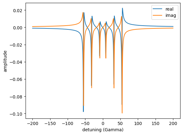
Amplitude Spectrum
The AmplitudeSpectrum is very similar to an energy spectrum but instead of intensities it provides complex amplitudes.
Amplitude methods are of Measurement type, cannot be fit to experimental data, and are intended for theoretical calculations.
Therefore, all experimental parameters of the FitMeasurement are not available.
Thickness or angular distributions cannot be applied because they assume incoherent addition of intensities.
The specific parameters for an amplitude spectrum are:
experiment: Experiment for the calculation.detuning: List with detuning values in units of the natural linewidth \(\Gamma\).electronic: EitherTrueorFalse. If electronic isTrueboth electronic and nuclear scattering are taken into account. It should be used to simulate the proper transmission through the sample. It will result in an absorption spectrum. In case you are only interested in the nuclear scattering properties set this parameter toFalse. In this case pure electronic scattering will be subtracted, see What Nexus calculates. This will result in a pure nuclear emission spectrum.time_gate: An empty or two element list. If a two element list is passed these two values [start, stop] are taken as a time gating of the energy spectrum calculation. Given in ns. Default is an empty list. The spectrum is Fourier transformed to the time domain, then the time gate is applied, and transformed back to the energy domain. Time gating will result in a reshaping of the spectrum depending cut components. Please note the for a proper Fourier transform, the detuning range large, typically larger than 1000 \(\Gamma\), and the step size should be smaller 0.5 \(\Gamma\).New in version 1.0.1.
To calculate amplitude properties the beam has to have a valid Jones vector. See Beam section for more details.
The AmplitudeSpectrum returns an array of Jones vectors.
So each array has the shape (detuning points, 2) with complex entries.
The first complex entry along the second dimension corresponds to the \(\sigma\) component, the second to the \(\pi\) component of the scattered field.
import nexus as nx
import numpy as np
import matplotlib.pyplot as plt

iron = nx.Material.Template(nx.lib.material.Fe)

layer_Fe = nx.Layer(id = "Fe layer",
                    material = iron,
                    thickness = 3000)

site = nx.Hyperfine(magnetic_field = 33,
                    isotropic = True)

iron.hyperfine_sites = [site]

sample = nx.Sample(layers = [layer_Fe])

beam = nx.Beam()
beam.LinearSigma()

exp = nx.Experiment(beam = beam,
                    objects = [sample],
                    isotope = nx.lib.moessbauer.Fe57)

detuning = np.linspace(-200, 200, 1001)

amp_spectrum = nx.AmplitudeSpectrum(experiment = exp,
                                    detuning = detuning,
                                    electronic = False,
                                    id = "my anplitude spectrum")

amp = amp_spectrum.Calculate()

amp_sigma = amp[:,0]
amp_pi = amp[:,1]

plt.plot(detuning, np.real(amp_sigma), label = 'real')
plt.plot(detuning, np.imag(amp_sigma), label = 'imag')
plt.legend()
plt.xlabel('detuning (Gamma)')
plt.ylabel('amplitude')
plt.show()
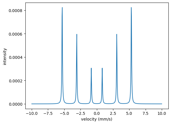
Moessbauer Spectrum
A classical Moessbauer spectrum is calculated by the MoessbauerSpectrum class.
It is an EnergySpectrum object with special initialization parameters.
The Doppler velocities are given for this method instead of detuning values in units of \(\Gamma\).
The convolution of the experimental data is done with a Lorentzian kernel, which accounts for the single line distribution of the Moessbauer source. It is set to the natural linewidth of one \(\Gamma\) of the source. Note, that standard kernel type in Nexus is Gaussian. The convolution of a Gaussian kernel and a Lorentzian resonance will result in a Voigt profile. To account for the Lorentzian profile of the Moessbauer source, the convolution kernel is set to a Lorentzian here.
You can specify the standard parameters for a FitMeasurement, see Measurements.
The specific parameters for the MoessbauerSpectrum are
velocity: List with velocities of the Moessbauer drive in mm/s.intensity_data: List of intensities measured during the experiment. Only needed for fitting.time_gate: An empty or two element list. If a two element list is passed these two values [start, stop] are taken as a time gating of the energy spectrum calculation. Given in ns. Default is an empty list. The spectrum is Fourier transformed to the time domain, then the time gate is applied, and transformed back to the energy domain. Time gating will result in a reshaping of the spectrum depending cut components. Please note the for a proper Fourier transform, the detuning range large, typically larger than 1000 \(\Gamma\), and the step size should be smaller 0.5 \(\Gamma\). This option will not results in a time gated Moessbauer spectrum.New in version 1.0.1.
Here is the code block of the Hello Nexus example again.
import nexus as nx
import numpy as np
import matplotlib.pyplot as plt

iron = nx.Material.Template(nx.lib.material.Fe)

layer_Fe = nx.Layer(id = "Fe layer",
                    material = iron,
                    thickness = 3000)

site = nx.Hyperfine(magnetic_field = 33,
                    isotropic = True)

iron.hyperfine_sites = [site]

sample = nx.Sample(layers = [layer_Fe])

beam = nx.Beam(polarization = 0)

exp = nx.Experiment(beam = beam,
                    objects = [sample],
                    isotope = nx.lib.moessbauer.Fe57)

velocities = np.linspace(-10, 10, 512)

moessbauer_spectrum = nx.MoessbauerSpectrum(experiment = exp,
                                            velocity = velocities)

intensity = moessbauer_spectrum.Calculate()

plt.plot(velocities, intensity)
plt.show()
As written before, the MoessbauerSpecrum is an EnergySpectrum with special parameters.
A Moessbauer spectrum can also be calculated from the EnergySpectrum directly with the following parameters.
detuning  = nx.VelocityToGamma(velocity, isotope)

moessbauer_spectrum = EnergySpectrum(experiment = exp,
                                     detuning = detuning,
                                     electronic = False,
                                     intensity_data = ...,
                                     scaling = ...,
                                     background = ...,
                                     resolution = 1.0,
                                     distribution_points = ...,
                                     fit_weight = ...,
                                     kernel_type = "Lorentz",
                                     residual = ...,
                                     time_gate = [],
                                     id = "...")

intensity = moessbauer_spectrum.Calculate()
Emission Spectrum
Warning
The theory of incoherent emission from internal conversion processes is not yet included. The method calculates the coherent scattering, subtracts the background and inverts the spectrum. Thus the full treatment of absorption of fluorescent X-rays or conversion electron electrons is not included.
Emission spectrum (from fluorescent X-rays or conversion electrons) is calculated by the EmissionSpectrum class.
It is a derived method from the EnergySpectrum class.
Note
For an emission spectrum the penetration depths of the detected entity must be accounted for. An X-ray fluorescence spectrum originates from several tens of \(\mu m\) while, a conversion electron Moessbauer spectrum (CEMS) only originates from a few tens of nm region near the surface. However, Nexus calculates the photon field behind the sample and will take electronic and nuclear scattering of all layers and the photon propagation along the sample into account. Therefore, you should only specify layers up to the approximate penetration depth (a few tens of nm for electrons and a few tens of \(\mu m\) for K-shell fluorescence). So, do not use the real sample layer structure or thickness if the accumulated length is larger then the penetration depth of the detected radiation. Otherwise the emission spectra might be wrong due to photon propagation effects along the sample or false contributions from not detectable layers.
The penetration depth depends on the energy of the conversion X-rays and electrons. For Fe-57, the 14.4 keV conversion process proceeds via ejection of a K-shell electron with a binding energy of 7.112 keV. Thus, conversion electrons have an energy of 14.4 keV - 7.1 keV = 7.3 keV. The K-shell is filled by an electron from the L-shell and this transition emits a \(K \alpha\) 6.4 keV X-ray. The 6.4 keV X-ray can leave the atom or create an Auger process leading to 5.6 keV electrons. Several other internal less probable processes are present.
See also
https://en.wikipedia.org/wiki/Conversion_electron_M%C3%B6ssbauer_spectroscopy
https://en.wikipedia.org/wiki/Internal_conversion
https://en.wikipedia.org/wiki/Internal_conversion_coefficient
The Doppler velocities are given for this method instead of detuning values in units of \(\Gamma\).
The convolution of the experimental is done with a Lorentzian kernel, which accounts for the single line distribution of the Moessbauer source. It is set to the natural linewidth of one \(\Gamma\) of the source. Note, that standard kernel type in Nexus is Gaussian. The convolution of a Gaussian kernel and a Lorentzian resonance will result in a Voigt profile. To account for the Lorentzian profile of the Moessbauer source, the convolution kernel is set to a Lorentzian here.
You can specify the standard parameters for a FitMeasurement, see Measurements.
The specific parameters for the Emissionpectrum are
velocity: List with velocities of the Moessbauer drive in mm/s.intensity_data: List of intensities measured during the experiment. Only needed for fitting.time_gate: An empty or two element list. If a two element list is passed these two values [start, stop] are taken as a time gating during spectrum collection. Given in ns. Default is an empty list. Time gating will results in a reshaping of the spectrum depending on the cut temporal components.
The calculation of an emission S is very similar to the one of a Moessbauer Spectrum. Here, a CEMS spectrum of a 10 nm film is calculated.
import nexus as nx
import numpy as np
import matplotlib.pyplot as plt

iron = nx.Material.Template(nx.lib.material.Fe)

# a 10 nm film is used for CEMS
layer_Fe = nx.Layer(id = "Fe layer",
                    material = iron,
                    thickness = 10)

site = nx.Hyperfine(magnetic_field = 33,
                    isotropic = True)

iron.hyperfine_sites = [site]

sample = nx.Sample(layers = [layer_Fe])

beam = nx.Beam()
beam.LinearSigma()

exp = nx.Experiment(beam = beam,
                    objects = [sample],
                    isotope = nx.lib.moessbauer.Fe57)

velocities = np.linspace(-10, 10, 512)

cem_spectrum = nx.EmissionSpectrum(experiment = exp,
                                   velocity = velocities)

intensity = cem_spectrum.Calculate()

plt.plot(velocities, intensity)
plt.xlabel('velocity (mm/s)')
plt.ylabel('intensity')
plt.show()
Time Spectrum
The TimeSpectrum is used to calculate the time dependent intensity of an experiment.
Actually, a quantum beat, originating from the hyperfine split lines, is measured.
It is often referred to as time spectrum in the NRS community.
You can specify the standard parameters for a FitMeasurement, see Measurements.
The specific parameters for the TimeSpectrum are
time_length: Sets the total length for the calculation of theTimeSpectrumin nanoseconds. For fits this value should be equal or larger than the measured time length.time_step: Sets the step size for the calculation of theTimeSpectrumin nanoseconds. The time steps should be reasonably chosen when fitting. A good time step is smaller than the measured time steps.max_detuning: Maximum value of the energy detuning (\(\Gamma\)) used for the internal energy representation during calculations. This value is 400 \(\Gamma\) on default. In case you expect nuclear features close or beyond this detuning increase the value. Larger values will decrease the computational speed. This option is mainly used for data fitting. For theoretical calculations set it to zero. Then, no cut in the energy domain is used and Nexus will take a large detuning range determined by the time settings. If this parameter is not zero, data beyondmax_detuningare padded to achieve the user time settings. To reduce padding effects, a window function is applied during the Fourier transformation, seefft_window.electronic: EitherTrueorFalse(default). If electronic isTrue, electronic and nuclear scattering are taken into account. For a time spectrum it will result in a large intensity at time zero due to the prompt electronic scattering. The default value isFalseas you are mostly interested in the delayed nuclear signal only, see What Nexus calculates.bunch_spacing: The bunch spacing of the synchrotron in nanoseconds. If provided, signals from previous bunches will be added to the time spectrum to account for all contributing signals to the measured time spectrum. The time_length is cut to the bunch spacing if it is larger.time_data: List of the experimental time values (nanoseconds). Only used for fitting.intensity_data: List of the experimental intensities. Only used for fitting.fft_window: A window function applied before the Fourier transformation. On default, Nexus automatically selects a Hann window whenmax_detuningis not0and no window when it is0. The options areauto(default) - will pick a Hann window ifmax_detuningis not zero, no window otherwise.HannHammingSineWelchKaiser2Kaiser window with \(\alpha = 2\)Kaiser25Kaiser window with \(\alpha = 2.5\)Kaiser3Kaiser window with \(\alpha = 3\)none
import nexus as nx
import numpy as np
import matplotlib.pyplot as plt

iron = nx.Material.Template(nx.lib.material.Fe)

layer_Fe = nx.Layer(id = "Fe layer",
                    material = iron,
                    thickness = 3000)

site = nx.Hyperfine(magnetic_field = 33,
                    magnetic_theta = 90,
                    magnetic_phi = 0,
                    quadrupole = 0.6)

site.SetRandomDistribution("efg", "3D", 401)

iron.hyperfine_sites = [site]

sample = nx.Sample(layers = [layer_Fe])

beam = nx.Beam()
beam.LinearSigma()

exp = nx.Experiment(beam = beam,
                    objects = [sample],
                    isotope = nx.lib.moessbauer.Fe57)

time_spectrum = nx.TimeSpectrum(experiment = exp,
                                time_length = 200,
                                time_step = 0.2,
                                bunch_spacing = 192.2, # PETRA III bunch spacing
                                id = "my time spectrum")

timeaxis, intensity = time_spectrum.Calculate()

plt.semilogy(timeaxis, intensity)
plt.xlabel('time (ns)')
plt.ylabel('intensity ($\Gamma$/ns)')
plt.show()
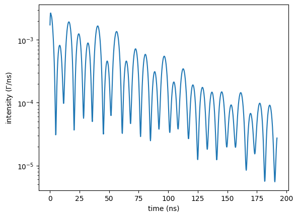
Note
In case electronic is set to True, the peak intensity at time zero depends on the time settings.
It is not to real scale with the nuclear scattering.
You can also ask for the detuning grid on which the scattering matrices are calculated via
print(np.array(time_spectrum.detuning))
When you want to know the detuning grid actually used for the FFT, set the maximum detuning also to zero.
time_spectrum.max_detuning = 0
print(np.array(time_spectrum.detuning))
When max_detuning is not zero, the scattering matrices at largest calculated detuning are padded to this detuning grid.
Time Spectrum Amplitude
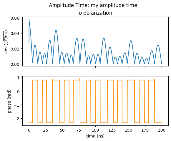
The AmplitudeTime is very similar to an time spectrum but instead of intensities it provides complex amplitudes.
Amplitude methods are of Measurement type, cannot be fit to experimental data, and are intended for theoretical calculations.
Therefore, all experimental parameters of the FitMeasurement are not available.
Thickness or angular distributions cannot be applied because they assume incoherent addition of intensities.
The specific parameters for an amplitude time spectrum are:
time_length: Sets the total length for the calculation of theTimeSpectrumin nanoseconds.time_step: Sets the step size for the calculation of theTimeSpectrumin nanoseconds.electronic: EitherTrueorFalse. If electronic isTrueelectronic and nuclear scattering are taken into account. For an amplitude time spectrum it will result in a large intensity at time zero due to the prompt electronic scattering. The default value isFalseas you are mostly interested in the delayed nuclear signal only, see What Nexus calculates.
To calculate amplitude properties the beam has to have a valid Jones vector defined. See, the tutorial section Beam for more details.
The AmplitudeTime returns an array of Jones vectors.
So each array has the shape (time_axis_points, 2) with complex entries.
The first complex entry along the second dimension corresponds to the \(\sigma\) component, the second to the \(\pi\) component of the scattered field.
import nexus as nx
import numpy as np
import matplotlib.pyplot as plt

iron = nx.Material.Template(nx.lib.material.Fe)

layer_Fe = nx.Layer(id = "Fe layer",
                    material = iron,
                    thickness = 3000)

site = nx.Hyperfine(magnetic_field = 33,
                    isotropic = True)

iron.hyperfine_sites = [site]

sample = nx.Sample(layers = [layer_Fe])

beam = nx.Beam()
beam.LinearSigma()

exp = nx.Experiment(beam = beam,
                    objects = [sample],
                    isotope = nx.lib.moessbauer.Fe57)

detuning = np.linspace(-200, 200, 1001)

amp_time = nx.AmplitudeTime(experiment = exp,
                            time_length = 200,
                            time_step = 0.2,
                            electronic = False,
                            id = "my amplitude time")

time_axis, amp = amp_time.Calculate()

amp_sigma = amp[:,0]
amp_pi = amp[:,1]

amp_time.Plot(sigma=True, pi=False, polar=True, unwrap=False)
Electronic properties of the experiment
These methods calculate properties of pure electronic scattering.
Typically, electronic scattering is considered without any polarization dependence, here however, polarization analyzers (Analyzer) or optically active elements (FixedObject) can also be included.
All methods described here are of Measurement type, cannot be fit to experimental data, and are intended for theoretical calculations.
Therefore, all experimental parameters of the FitMeasurement are not available.
The only parameter you have to specify for all methods, except the experiment, is:
energy: The photon energy for the calculation in eV.
Amplitudes
The Amplitudes method provides the complex scattering amplitude behind each object in the experiment.
The Amplitudes method is not dependent on the polarization state.
Only the scattering factors are calculated.
For Analyzers and FixedObjects the provided scattering_factor is used.
import nexus as nx
import numpy as np
import matplotlib.pyplot as plt

iron = nx.Material.Template(nx.lib.material.Fe)

layer_Fe = nx.Layer(id = "Fe layer",
                    material = iron,
                    thickness = 3000)

sample1 = nx.Sample(layers = [layer_Fe])

layer_Pt = nx.Layer(id = "Pt layer",
                    material = nx.Material.Template(nx.lib.material.Pt),
                    thickness = 1000)

sample2 = nx.Sample(layers=[layer_Pt])

beam = nx.Beam()
beam.LinearSigma()

exp = nx.Experiment(beam = beam,
                    objects = [sample1, sample2],
                    isotope = nx.lib.moessbauer.Fe57)

electronic_amplitudes = nx.Amplitudes(experiment = exp,
                                      energy = 14400)

print(electronic_amplitudes())
Here you will get a list with two complex numbers [0.73356471-0.57043914j 0.67507685+0.37599394j] each corresponding to the amplitude of the photon field behind each sample.
The input field in Nexus is assumed to be 1+j0.
After the first sample the field amplitude is 0.73356471-0.57043914j and after the second sample it is 0.67507685+0.37599394j.
Matrices
The Matrices method provides the accumulated complex scattering matrix up to each object in the experiment.
The Matrices method depends on the polarization state.
For Analyzers and FixedObjects the scattering matrices are used, i.e. the Analyzer.matrix and the FixedObject.matrix.
import nexus as nx
import numpy as np
import matplotlib.pyplot as plt

iron = nx.Material.Template(nx.lib.material.Fe)

layer_Fe = nx.Layer(id = "Fe layer",
                    material = iron,
                    thickness = 3000)

sample1 = nx.Sample(layers = [layer_Fe])

layer_Pt = nx.Layer(id = "Pt layer",
                    material = nx.Material.Template(nx.lib.material.Pt),
                    thickness = 1000)

sample2 = nx.Sample(layers=[layer_Pt])

beam = nx.Beam()
beam.LinearSigma()

exp = nx.Experiment(beam = beam,
                    objects = [sample1, sample2])

scattering_matrices = nx.Matrices(experiment = exp,
                                  energy = 14400)

print(scattering_matrices())
You will get two 2x2 matrices corresponding to the two accumulated scattering matrices up to each sample.
[[[0.73356471-0.57043914j 0.        +0.j        ]
  [0.        +0.j         0.73356471-0.57043914j]]

 [[0.67507685+0.37599394j 0.        +0.j        ]
  [0.        +0.j         0.67507685+0.37599394j]]]
Jones vectors
The JonesVectors method provides the complex Jones vector of the photon field behind each object in the experiment.
The JonesVectors method depends on the polarization state.
A proper Jones vector has to be set in the Beam object of the experiment.
For Analyzers and FixedObjects the scattering matrices are used, i.e. the Analyzer.matrix and the FixedObject.matrix.
import nexus as nx
import numpy as np
import matplotlib.pyplot as plt

iron = nx.Material.Template(nx.lib.material.Fe)

layer_Fe = nx.Layer(id = "Fe layer",
                    material = iron,
                    thickness = 3000)

sample1 = nx.Sample(layers = [layer_Fe])

layer_Pt = nx.Layer(id = "Pt layer",
                    material = nx.Material.Template(nx.lib.material.Pt),
                    thickness = 1000)

sample2 = nx.Sample(layers=[layer_Pt])

beam = nx.Beam()
beam.LinearSigma()

exp = nx.Experiment(beam = beam,
                    objects = [sample1, sample2])

jones_vectors = nx.JonesVectors(experiment = exp,
                                energy = 14400)

print(jones_vectors())

# now we add an analyzer
print("\nwith Pi analyzer")

analyzer  = nx.Analyzer()
analyzer.LinearPi()

exp.objects = [sample1, analyzer, sample2]

print(jones_vectors())
You will get complex entries corresponding to the Jones vectors behind each object.
[[0.73356471-0.57043914j 0.        +0.j        ]
 [0.67507685+0.37599394j 0.        +0.j        ]]

with Pi analyzer
[[0.73356471-0.57043914j 0.        +0.j        ]
 [0.        +0.j         0.        +0.j        ]
 [0.        +0.j         0.        +0.j        ]]
Intensities
The Intensities method provides the intensity of the photon field behind each object in the experiment.
The Intensities method depends on the polarization state.
For Analyzers and FixedObjects the scattering matrices are used, i.e. the Analyzer.matrix and the FixedObject.matrix.
import nexus as nx
import numpy as np
import matplotlib.pyplot as plt

iron = nx.Material.Template(nx.lib.material.Fe)

layer_Fe = nx.Layer(id = "Fe layer",
                    material = iron,
                    thickness = 3000)

sample1 = nx.Sample(layers = [layer_Fe])

layer_Pt = nx.Layer(id = "Pt layer",
                    material = nx.Material.Template(nx.lib.material.Pt),
                    thickness = 1000)

sample2 = nx.Sample(layers=[layer_Pt])

beam = nx.Beam()
beam.LinearSigma()

exp = nx.Experiment(beam = beam,
                    objects = [sample1, sample2])

intensities = nx.Intensities(experiment = exp,
                             energy = 14400)

print(intensities())
You will get [0.863518 0.5971002] corresponding to the two field intensities behind each sample.
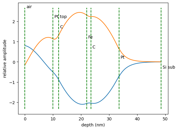
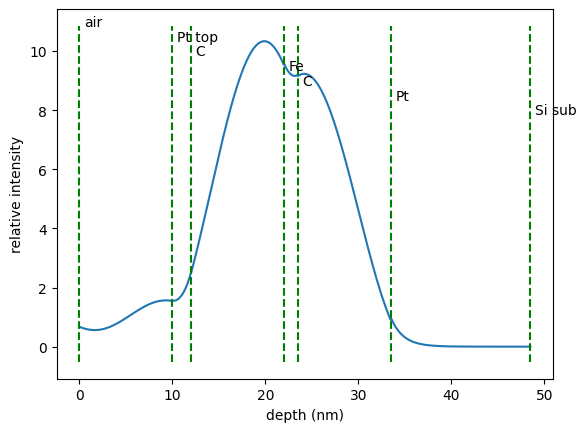
Fields inside a sample
The FieldAmplitudes and Field Intensity methods calculate the field inside a sample.
Both methods are of Measurement type, cannot be fit to experimental data, and are intended for theoretical calculations.
Therefore, all experimental parameters of the FitMeasurement are not available.
Both methods do not take an experiment but only a sample as argument. The methods work for forward and grazing-incidence scattering. The specific parameters for a field amplitude are:
sample: The sample for which the field should be calculated.energy: The photon energy for the calculation in eV.points: Number of points to calculate the field inside the sample.
The methods are not dependent on the polarization state. Only the scattering factor is calculated.
In this example we create a thin-film cavity structure. We also add an air layer to calculate the field above the cavity.
import nexus as nx
import numpy as np
import matplotlib.pyplot as plt

# --------------------- air --------------
lay_air = nx.Layer(id = "air",
                   material = nx.Material.Template(nx.lib.material.air),
                   thickness = 10,
                   roughness = 0)

# ------------------------- Fe layer --------------------------
lay_Fe = nx.Layer(id = "Fe",
                  material = nx.Material.Template(nx.lib.material.Fe_enriched),
                  thickness = 1.5,
                  roughness = 0.35)

# ----------------------------- Pt layers -----------------------------
lay_Pt_top = nx.Layer(id = "Pt top",
                      material = nx.Material.Template(nx.lib.material.Pt),
                      thickness = 2,
                     roughness = 0.2)

lay_Pt = nx.Layer(id = "Pt",
                material = nx.Material.Template(nx.lib.material.Pt),
                thickness = 15,
                roughness = 0.77)

# -------------------------- C layer ---------------------------
lay_C = nx.Layer(id = "C",
                material = nx.Material.Template(nx.lib.material.C),
                thickness = 10,
                roughness = 0.3)

# --------------------- substrate ---------------------------------
lay_substrate = nx.Layer(id = "Si sub",
                material = nx.Material.Template(nx.lib.material.Si),
                thickness = nx.inf,
                roughness = 0.4)

# --------------------- sample ---------------------------------
sample = nx.Sample(id = "simple layers",
                   layers = [lay_air,
                             lay_Pt_top,
                             lay_C,
                             lay_Fe,
                             lay_C,
                             lay_Pt,
                             lay_substrate],
                    geometry = "r",
                    angle = 0.161, # at the sample.angle the field will be calculated
                    length = 10,
                    roughness = "a")

beam  = nx.Beam(fwhm = 0)

exp = nx.Experiment(beam = beam,
                    objects = [sample],
                    isotope = nx.moessbauer.Fe57,
                    id = "my exp")

field_amps = nx.FieldAmplitude(sample = sample,
                               energy = nx.moessbauer.Fe57.energy,
                               points = 1001)

depth, amp = field_amps.Calculate()

plt.plot(depth, np.real(amp))
plt.plot(depth, np.imag(amp))

# add lines and labels
axes = plt.gca()
y_min, y_max = axes.get_ylim()
plt.vlines(sample.Interfaces(), y_min, y_max, colors='g', linestyles='dashed')
for id, location in zip(sample.Ids(), np.array(sample.Interfaces()) + 0.5):
    plt.text(location, y_max, id, fontsize = 10)
    y_max = y_max - 0.5

plt.xlabel('depth (nm)')
plt.ylabel('relative amplitude')
plt.show()

field_int = nx.FieldIntensity(sample = sample,
                              energy = nx.moessbauer.Fe57.energy,
                              points = 1001)

depth, int = field_int()

plt.plot(depth, int)

# add lines and labels
axes = plt.gca()
y_min, y_max = axes.get_ylim()
plt.vlines(sample.Interfaces(), y_min, y_max, colors='g', linestyles='dashed')
for id, location in zip(sample.Ids(), np.array(sample.Interfaces()) + 0.5):
    plt.text(location, y_max, id, fontsize = 10)
    y_max = y_max - 0.5

plt.xlabel('depth (nm)')
plt.ylabel('relative intensity')
plt.show()
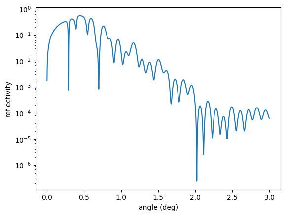
Reflectivity and Transmission
The Reflectivity and Transmission methods calculate the mentioned method in grazing incidence geometry.
You can specify the standard parameters for a FitMeasurement, see Measurements.
The convolution with the resolution parameter is done on the angular values. So the resolution is an angular resolution (degree).
The specific parameters for the two methods are
sample: Sample objects of the experiment whose angle is changed. Only one sample can have a changing angle.energy: X-ray energy in eV.angles: List of the angles for which the reflectivity or transmission is calculated in degree.intensity_data: List of the experimental intensities. Only used for fitting.
In this example we create a thin-film cavity structure and calculate both methods.
import nexus as nx
import numpy as np
import matplotlib.pyplot as plt
# ------------------------- Fe layer --------------------------
lay_Fe = nx.Layer(id = "Fe",
material = nx.Material.Template(nx.lib.material.Fe_enriched),
thickness = 1.5,
roughness = 0.35)
# ----------------------------- Pt layers -----------------------------
lay_Pt_top = nx.Layer(id = "Pt top",
material = nx.Material.Template(nx.lib.material.Pt),
thickness = 2,
roughness = 0.2)
lay_Pt = nx.Layer(id = "Pt",
material = nx.Material.Template(nx.lib.material.Pt),
thickness = 15,
roughness = 0.77)
# -------------------------- C layer ---------------------------
lay_C = nx.Layer(id = "C",
material = nx.Material.Template(nx.lib.material.C),
thickness = 10,
roughness = 0.3)
# --------------------- substrate ---------------------------------
lay_substrate = nx.Layer(id = "Si sub",
material = nx.Material.Template(nx.lib.material.Si),
thickness = nx.inf,
roughness = 0.4)
# --------------------- sample ---------------------------------
# is defined in reflection here
sample = nx.Sample(id = "simple layers",
layers = [lay_Pt_top,
lay_C,
lay_Fe,
lay_C,
lay_Pt,
lay_substrate],
geometry = "r",
length = 10,
roughness = "a")
beam = nx.Beam(fwhm = 0.2)
exp = nx.Experiment(beam = beam,
objects = [sample],
id = "my exp")
angles = np.arange(0.001, 3, 0.001)
reflectivity = nx.Reflectivity(experiment = exp,
sample = sample,
energy = nx.lib.energy.CuKalpha, # Cu K alpha line
angles = angles,
resolution = 0.001)
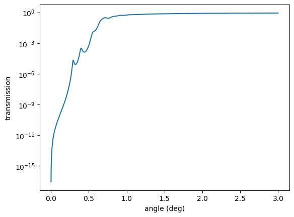
plt.semilogy(angles, reflectivity())
plt.xlabel('angle (deg)')
plt.ylabel('reflectivity')
plt.show()
# remove the infinite substrate and set to transmission geometry
sample.layers = [lay_Pt_top,
lay_C,
lay_Fe,
lay_C,
lay_Pt]
sample.geometry = "t"
transmission = nx.Transmission(experiment = exp,
sample = sample,
energy = nx.lib.energy.CuKalpha, # Cu K alpha line
angles = angles,
resolution = 0.001)
plt.semilogy(angles, transmission())
plt.xlabel('angle (deg)')
plt.ylabel('transmission')
plt.show()
Reflectivity and Transmission Amplitudes
The ReflectivityAmplitude and TransmissionAmplitude methods calculate the complex amplitudes in grazing incidence geometry.
Amplitude methods are of Measurement type, cannot be fit to experimental data, and are intended for theoretical calculations.
Therefore, all experimental parameters of the FitMeasurement are not available.
The specific parameters for the two methods are
sample: Sample objects of the experiment whose angle is changed. Only one sample can have a changing angle.energy: X-ray energy in eV.angles: List of the angles for which the reflectivity is calculated in degree.
In this example we create a thin-film cavity structure and calculate both methods.
import nexus as nx
import numpy as np
import matplotlib.pyplot as plt
# ------------------------- Fe layer --------------------------
lay_Fe = nx.Layer(id = "Fe",
material = nx.Material.Template(nx.lib.material.Fe_enriched),
thickness = 1.5,
roughness = 0.35)
# ----------------------------- Pt layers -----------------------------
lay_Pt_top = nx.Layer(id = "Pt top",
material = nx.Material.Template(nx.lib.material.Pt),
thickness = 2,
roughness = 0.2)
lay_Pt = nx.Layer(id = "Pt",
material = nx.Material.Template(nx.lib.material.Pt),
thickness = 15,
roughness = 0.77)
# -------------------------- C layer ---------------------------
lay_C = nx.Layer(id = "C",
material = nx.Material.Template(nx.lib.material.C),
thickness = 10,
roughness = 0.3)
# --------------------- substrate ---------------------------------
lay_substrate = nx.Layer(id = "Si sub",
material = nx.Material.Template(nx.lib.material.Si),
thickness = nx.inf,
roughness = 0.4)
# --------------------- sample ---------------------------------
# is defined in reflection here
sample = nx.Sample(id = "simple layers",
layers = [lay_Pt_top,
lay_C,
lay_Fe,
lay_C,
lay_Pt,
lay_substrate],
geometry = "r",
length = 10,
roughness = "a")
beam = nx.Beam(fwhm = 0.2)
exp = nx.Experiment(beam = beam,
objects = [sample],
id = "my exp")
angles = np.arange(0.001, 3, 0.001)
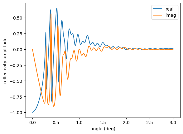
reflectivity_amp = nx.ReflectivityAmplitude(experiment = exp,
sample = sample,
energy = nx.lib.energy.CuKalpha, # Cu K alpha line
angles = angles)
ref = reflectivity_amp()
plt.plot(angles, np.real(ref), label='real')
plt.plot(angles, np.imag(ref), label='imag')
plt.legend()
plt.xlabel('angle (deg)')
plt.ylabel('reflectivity amplitude')
plt.show()
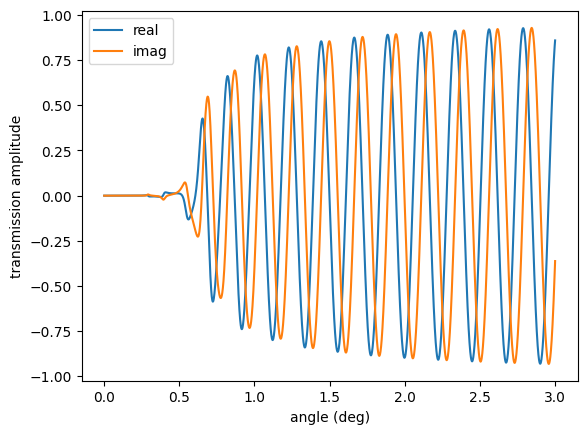
# remove the infinite substrate and set to transmission geometry
sample.layers = [lay_Pt_top,
lay_C,
lay_Fe,
lay_C,
lay_Pt]
sample.geometry = "t"
transmission_amp = nx.TransmissionAmplitude(experiment = exp,
sample = sample,
energy = nx.lib.energy.CuKalpha, # Cu K alpha line
angles = angles)
trans = transmission_amp()
plt.plot(angles, np.real(trans), label='real')
plt.plot(angles, np.imag(trans), label='imag')
plt.legend()
plt.xlabel('angle (deg)')
plt.ylabel('transmission amplitude')
plt.show()
Nuclear Reflectivities
The NuclearReflectivity and NuclearReflectivityEnergy methods calculate the reflected intensity in grazing incidence geometry.
The NuclearReflectivity gives the time-integrated delayed scattered radiation, so the integrated time spectrum at each angle.
So, electronic scattering is typically not observed due to the veto set in a time spectrum.
The NuclearReflectivityEnergy gives the energy-integrated delayed scattered radiation, so the integrated energy spectrum at each angle.
Here, electronic scattering is included. This method should be used to simulate or fit data from a synchrotron Moessbauer source (SMS).
You can specify the standard parameters for a FitMeasurement, see Measurements.
The convolution with the resolution parameter is done on the angular values. So the resolution is an angular resolution (degree).
The specific parameters common for the two methods are
sample: Sample objects of the experiment whose angle is changed. Only one sample can have a changing angle.energy: X-ray energy in eV.angles: List of the angles for which the reflectivity is calculated in degree.intensity_data: List of the experimental intensities. Only used for fitting.
For NuclearReflectivityEnergy the additional parameters are
detuning: Detuning range over which the integration takes place.time_gate: An empty or two element list. If a two element list is passed these two values [start, stop] are taken as a time gating of the energy spectrum calculation. Given in ns. Default is an empty list. The spectrum is Fourier transformed to the time domain, then the time gate is applied, and transformed back to the energy domain. Time gating will result in a reshaping of the spectrum depending cut components. Please note the for a proper Fourier transform, the detuning range large, typically larger than 1000 \(\Gamma\), and the step size should be smaller 0.5 \(\Gamma\).
For NuclearReflectivity the additional parameters are
time_start: Start time for the integration (ns).time_stop: Stop time for the integration (ns).time_step: Step size for the time axis (ns).max_detuning: Maximum value of the energy detuning (\(\Gamma\)) used for the internal energy representation during calculations. This value is 400 \(\Gamma\) on default. In case you expect nuclear features close or beyond this detuning increase the value. Larger values will decrease the computational speed. When you don’t want to use a cut in the energy space set this value to0. Then, Nexus will calculate a large detuning range determined by the time settings.
In this example we create a thin-film cavity structure and calculate both methods.
import nexus as nx
import numpy as np
import matplotlib.pyplot as plt
# ------------------------- Fe layer --------------------------
mat_Fe = nx.Material.Template(nx.lib.material.Fe_enriched)
site = nx.Hyperfine(magnetic_field = 33,
magnetic_theta = 90,
magnetic_phi = 0)
mat_Fe.hyperfine_sites = [site]
lay_Fe = nx.Layer(id = "Fe",
material = mat_Fe,
thickness = 1.5,
roughness = 0.35)
# ----------------------------- Pt layers -----------------------------
lay_Pt_top = nx.Layer(id = "Pt top",
material = nx.Material.Template(nx.lib.material.Pt),
thickness = 2,
roughness = 0.2)
lay_Pt = nx.Layer(id = "Pt",
material = nx.Material.Template(nx.lib.material.Pt),
thickness = 15,
roughness = 0.77)
# -------------------------- C layer ---------------------------
lay_C = nx.Layer(id = "C",
material = nx.Material.Template(nx.lib.material.C),
thickness = 10,
roughness = 0.3)
# --------------------- substrate ---------------------------------
lay_substrate = nx.Layer(id = "Si sub",
material = nx.Material.Template(nx.lib.material.Si),
thickness = nx.inf,
roughness = 0.4)
# --------------------- sample ---------------------------------
# is defined in reflection here
sample = nx.Sample(id = "simple layers",
layers = [lay_Pt_top,
lay_C,
lay_Fe,
lay_C,
lay_Pt,
lay_substrate],
geometry = "r",
length = 10,
roughness = "a")
beam = nx.Beam(fwhm = 0.2)
exp = nx.Experiment(beam = beam,
objects = [sample],
isotope = nx.lib.moessbauer.Fe57,
id = "my exp")
angles = np.arange(0.01, 1, 0.01)
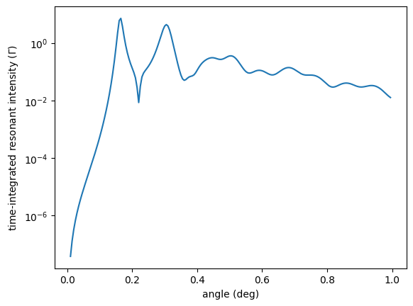
nuc_ref = nx.NuclearReflectivity(experiment = exp,
sample = sample,
angles = angles,
time_start = 10,
time_stop = 192,
time_step = 0.2,
max_detuning = 400,
intensity_data = [],
scaling = "auto",
background = 0,
fit_weight = 1.0,
resolution = 0.001)
plt.semilogy(angles, nuc_ref())
plt.xlabel('angle (deg)')
plt.ylabel('time-integrated resonant intensity ($\Gamma$)')
plt.show()
Here you will get some warnings
-------------------------------------------------------------------------------------------
 NEXUS WARNING in NuclearReflectivity
 warning: Analytical roughness model of interface W matrix not valid! Output might be wrong!
          At angle 0.990000 and at energy 14412.497000.
          Wavevector kz * roughness.value = 0.378586 > 0.3 but should be << 1.
          Encountered in Sample.id:   - Layer.id: C  - Layer.roughness: 0.300000
-------------------------------------------------------------------------------------------
which tell you to be careful with the calculated nuclear reflectivity as the model on the roughness is quite stressed.
You can see that the values of Wavevector kz * roughness.value are about 0.38 at an incidence angle of 0.99 degree.
The model might still be OK but its is always the users responsibility to check this.
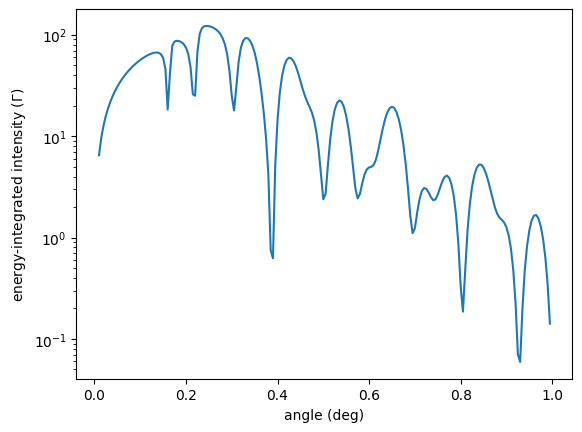
The NuclearReflectivityEnergy is similar. It is the reflectivity that one obtains when using a synchrotron Moessbauer source (SMS).
detuning = np.linspace(-200, 200, 1001)

nuc_ref = nx.NuclearReflectivityEnergy(experiment = exp,
                                       sample = sample,
                                       angles = angles,
                                       detuning = detuning,
                                       intensity_data = [],
                                       scaling = "auto",
                                       background = 0,
                                       fit_weight = 1.0,
                                       resolution = 0.001,
                                       time_gate = [])

plt.semilogy(angles, nuc_ref())
plt.xlabel('angle (deg)')
plt.ylabel('energy-integrated intensity ($\Gamma$)')
plt.show()
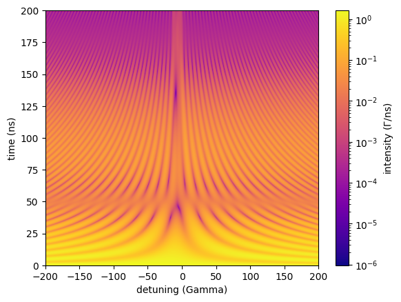
Energy Time Spectrum
The EnergyTimeSpectrum method calculates the time dependent intensity for different energy detunings of one sample in the experiment.
The sample is assumed to be Doppler shifted on some kind of mechanical drive (Doppler detuning).
The momentary detuning that is specified will lead to an energetic shift of the transition on the moved sample.
Thus, an interferogram of the shifted transitions with respect to all other transitions in the experiment is calculated.
You can specify the standard parameters for a FitMeasurement, see Measurements. The specified energy resolution is not that of a source like in a Moessbauer spectrum because here a broadband excitation with a synchrotron pulse is assumed. The energy resolution is any additional broadening term, like noise on the drive motion for example. The time resolution is the one of the temporal detector, i.e. an APD.
The specific parameters for the EnergySpectrum are
time_length: Length of the calculation (ns).time_step: Step size of the calculation in (ns). This should be smaller than the experimentaltime_datastep size.mode: Identifier for the calculation mode.i- interpolate mode. The scattering properties are interpolated on the detuning values (recommended fast mode).f- full mode. The scattering properties at different detuning values are calculated via a change of the isomer shift (slow mode).
electronic: EitherTrueorFalse. If electronic isTrueboth electronic and nuclear scattering are taken into account. In case you are only interested in the nuclear delayed scattering properties set this parameter toFalse. In this case pure electronic scattering will be subtracted, see What Nexus calculates. This will result in a pure nuclear emission spectrum.time_data: Time axis of the intensity data. Only used for fitting.intensity_data: 2D intensity data used for fitting. The 1st dimension corresponds to the detuning, the 2nd to the time.
The returned array has the shape (detuning points, time steps).
import nexus as nx
import numpy as np
import matplotlib.pyplot as plt
from matplotlib import colors

# ----------------- cavity in reflection geometry -------------

# ------------------------- Fe layer --------------------------
lay_Fe = nx.Layer(id = "Fe",
                material = nx.Material.Template(nx.lib.material.Fe_enriched),
                thickness = 1.5,
                roughness = 0.3)

site1 = nx.Hyperfine(magnetic_field = 33)

lay_Fe.material.hyperfine_sites = [site1]

# ----------------------------- Pt layers -----------------------------
lay_Pt_top = nx.Layer(id = "Pt top",
                material = nx.Material.Template(nx.lib.material.Pt),
                thickness = 2,
                roughness = 0.3)

lay_Pt = nx.Layer(id = "Pt",
                material = nx.Material.Template(nx.lib.material.Pt),
                thickness = 15,
                roughness = 0.3)

# -------------------------- C ---------------------------
lay_C = nx.Layer(id = "C",
                material = nx.Material.Template(nx.lib.material.C),
                thickness = 10,
                roughness = 0.3)

# --------------------- substrate ---------------------------------
lay_substrate = nx.Layer(id = "Si sub",
                material = nx.Material.Template(nx.lib.material.Si),
                thickness = nx.inf,
                roughness = 0.3)

sample_cavity = nx.Sample(id = "simple layers",
                          layers = [lay_Pt_top,
                                    lay_C,
                                    lay_Fe,
                                    lay_C,
                                    lay_Pt,
                                    lay_substrate],
                           geometry = "r",
                           angle = 0.148,
                           roughness = "a")

# ------------- Stainless steel foil on a drive in forward geometry ----------------
foil = nx.Layer(id = "StainSteel",
                material = nx.Material.Template(nx.lib.material.SS_enriched),
                thickness = 3000)

site_foil = nx.Hyperfine(
    isomer = -0.09,  # with respect to iron
    quadrupole = 0.6,
    isotropic = True)

foil.material.hyperfine_sites = [site_foil]

sample_foil = nx.Sample(id = "simple foil ",
                        layers = [foil],
                        geometry = "f")

# define a detuning for the sample on the drive
sample_foil.drive_detuning = np.linspace(-200, 200, 1024)

# -------------------------- setup experiment ------------------------
beam  = nx.Beam()
beam.LinearSigma()

exp = nx.Experiment(beam = beam,
                    objects = [sample_cavity, sample_foil],
                    isotope = nx.moessbauer.Fe57,
                    id = "my exp")

energy_time_spec = nx.EnergyTimeSpectrum(experiment = exp,
                            time_length = 200.0,
                            time_step = 0.2,
                            mode = "i",
                            electronic = False)

timescale, intensity = energy_time_spec()

plt.imshow(intensity.T,
           cmap=plt.cm.plasma,
           norm=colors.LogNorm(),
           aspect='auto',
           origin='lower',
           extent=(min(sample_foil.drive_detuning), max(sample_foil.drive_detuning), min(timescale), max(timescale)))

plt.colorbar(orientation='vertical', label = 'intensity ($\Gamma$/ns)')
plt.xlabel('detuning (Gamma)')
plt.ylabel('time (ns)')
plt.show()
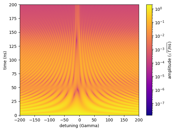
Energy Time Amplitude
The EnergyTimeAmplitude is very similar to an EnergyTimeSpectrum but instead of intensities it provides complex amplitudes.
Amplitude methods are of Measurement type, cannot be fit to experimental data, and are intended for theoretical calculations.
Therefore, all experimental parameters of the FitMeasurement are not available.
Thickness or angular distributions cannot be applied because they assume incoherent addition of intensities.
The specific parameters for an amplitude spectrum are:
time_length: Length of the calculation (ns).time_step: Step size of the calculation in (ns). This should be smaller than the experimentaltime_datastep size.mode: Identifier for the calculation mode.i- interpolate mode. The scattering properties are interpolated on the detuning values (recommended fast mode).f- full mode. The scattering properties at different detuning values are calculated via a change of the isomer shift (slow mode).
electronic: EitherTrueorFalse. If electronic isTrueboth electronic and nuclear scattering are taken into account. In case you are only interested in the nuclear delayed scattering properties set this parameter toFalse. In this case pure electronic scattering will be subtracted, see What Nexus calculates. This will result in a pure nuclear emission spectrum.
To calculate amplitude properties, the beam has to have a valid Jones vector. See, the Beam section for more details.
The EnergyTimeAmplitude returns a 2D array of Jones vectors.
So each array has the shape (detuning points, time steps, 2) with complex entries.
The first complex entry along the third dimension corresponds to the \(\sigma\) component, the second to the \(\pi\) component of the scattered field.
import nexus as nx
import numpy as np
import matplotlib.pyplot as plt
from matplotlib import colors

# ----------------- cavity in reflection geometry -------------

# ------------------------- Fe layer --------------------------
lay_Fe = nx.Layer(id = "Fe",
                material = nx.Material.Template(nx.lib.material.Fe_enriched),
                thickness = 1.5,
                roughness = 0.3)

site1 = nx.Hyperfine(magnetic_field = 0)

lay_Fe.material.hyperfine_sites = [site1]

# ----------------------------- Pt layers -----------------------------
lay_Pt_top = nx.Layer(id = "Pt top",
                material = nx.Material.Template(nx.lib.material.Pt),
                thickness = 2,
                roughness = 0.3)

lay_Pt = nx.Layer(id = "Pt",
                material = nx.Material.Template(nx.lib.material.Pt),
                thickness = 15,
                roughness = 0.3)

# -------------------------- C ---------------------------

lay_C = nx.Layer(id = "C",
                material = nx.Material.Template(nx.lib.material.C),
                thickness = 10,
                roughness = 0.3)

# --------------------- substrate ---------------------------------
lay_substrate = nx.Layer(id = "Si sub",
                material = nx.Material.Template(nx.lib.material.Si),
                thickness = nx.inf,
                roughness = 0.3)

sample_cavity = nx.Sample(id = "simple layers",
                          layers = [lay_Pt_top,
                                    lay_C,
                                    lay_Fe,
                                    lay_C,
                                    lay_Pt,
                                    lay_substrate],
                           geometry = "r",
                           angle = 0.148,
                           roughness = "a")

# ------------- Stainless steel foil in forward geometry ----------------
foil = nx.Layer(id = "StainSteel",
                material = nx.Material.Template(nx.lib.material.SS_enriched),
                thickness = 3000)

site_foil = nx.Hyperfine(
    isomer = -0.09,  # mm/s
    quadrupole = 0.6,
    isotropic = True)

foil.material.hyperfine_sites = [site_foil]

sample_foil = nx.Sample(id = "simple foil ",
                        layers = [foil],
                        geometry = "f")

beam  = nx.Beam()
beam.LinearSigma()

exp = nx.Experiment(beam = beam,
                    objects = [sample_cavity, sample_foil],
                    isotope = nx.moessbauer.Fe57,
                    id = "my exp")

# define a detuning for the sample on the drive
sample_foil.drive_detuning = np.linspace(-200, 200, 1024)  # Gamma

eta = nx.EnergyTimeAmplitude(experiment = exp,
                            time_length = 200.0,
                            time_step = 0.2,
                            mode = "i",
                            electronic = False)

timescale, amp = eta()

# calculate intensity from Jones vector
intensity = np.square(np.abs(amp[:,:,0])) + np.square(np.abs(amp[:,:,1]))

plt.imshow(intensity.T,
           cmap=plt.cm.plasma,
           norm=colors.LogNorm(),
           aspect='auto',
           origin = 'lower',
           extent=(min(sample_foil.drive_detuning), max(sample_foil.drive_detuning), min(timescale), max(timescale)))

plt.colorbar(orientation='vertical', label = 'amplitude ($\sqrt{\Gamma / \mathrm{ns}}$)')
plt.xlabel('detuning (Gamma)')
plt.ylabel('time (ns)')
plt.show()
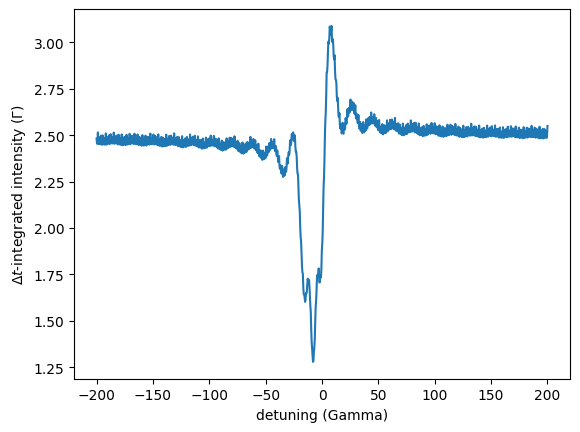
Integrated Energy Time Spectrum
The IntegratedEnergyTimeSpectrum method calculates the time integrated intensity of a EnergyTimeSpectrum.
Therefore, the two integration borders have to be specified in addition to the parameters of the EnergyTimeSpectrum.
integration_start: Start time of the integration (ns).integration_stop: Stop time of the integration (ns).
The intensity integration is done between the two values.
int_energy_time_spec = nx.IntegratedEnergyTimeSpectrum(experiment = exp,
                                                       time_length = 200.0,
                                                       time_step = 0.2,
                                                       integration_start = 51,
                                                       integration_stop = 180,
                                                       mode = "i",
                                                       electronic = False)

intensity = int_energy_time_spec()

plt.plot(sample_foil.drive_detuning, intensity)
plt.xlabel('detuning (Gamma)')
plt.ylabel('$\Delta t$-integrated intensity ($\Gamma$)')
plt.show()
Notebooks
energy spectrum - nb_energy_spectrum.ipynb.
energy spectrum time gate - nb_energy_spectrum_time_gate.ipynb.
amplitude spectrum - nb_amplitude_spectrum.ipynb.
emission spectrum - nb_emission_spectrum.ipynb.
time spectrum - nb_time_spectrum.ipynb.
amplitude time - nb_amplitude_time.ipynb.
amplitudes - nb_amplitudes.ipynb.
intensities - nb_intensities.ipynb.
JonesVector - nb_JonesVector.ipynb.
reflectivity - nb_reflectivity.ipynb.
reflectivity amplitudes - nb_reflectivity_amplitudes.ipynb.
nuclear reflectivity - nb_nuclear_reflectivity.ipynb.
energy time spectrum - nb_energy_time_spectrum.ipynb.
energy time amplitude - nb_energy_time_amplitude.ipynb.
Please have a look to the API Reference for more information.