Hyperfine parameters
The hyperfine parameters define the energy of the Hamiltonian for the different spin states of the nucleus. For a Moessbauer isotope one has to consider the isomer shift, the quadrupole splitting and the magnetic hyperfine field. The quantization system for the hyperfine parameters is set to the coordinates system of the beam
and all angles of the spherical hyperfine parameters are referenced to this coordinate system.
The following parameters are Var objects and can be fit for :class:`Hyperfine` site:
relative weight of the site
isomer shift
magnetic field
magnetic polar angle
magnetic azimuthal angle
quadrupole slitting
quadrupole ZYZ extrinsic Euler angle alpha
quadrupole ZYZ extrinsic Euler angle beta
quadrupole ZYZ extrinsic Euler angle gamma
quadrupole asymmetry
New in version 1.1.2.
texture
Lamb-Moessbauer factor
A Hyperfine object with all attributes defined looks like this
hyperfine = nx.Hyperfine(
   id = "example parameter",
   weight = 1,                  # relative weight of the site in the material
   isomer = -0.11,              # isomer shift in mm/s
   magnetic_field = 33,         # magnetic field in T
   magnetic_theta = 0,          # polar angle
   magnetic_phi = 45,           # azimuthal angle
   quadrupole = 0.8,            # quadrupole slitting in mm/s
   quadrupole_alpha = 90,       # ZYZ extrinsic Euler angle alpha
   quadrupole_beta = 45,        # ZYZ extrinsic Euler angle beta
   quadrupole_gamma = 0,        # ZYZ extrinsic Euler angle gamma
   quadrupole_asymmetry = 0.05, # Asymmetry parameter
   texture = 1.0,               # texture coefficient
   lamb_moessbauer = 1.0,       # site specific Lamb-Moessbauer factor
   isomer_dist = None,
   magnetic_field_dist = None,
   magnetic_theta_dist = None,
   magnetic_phi_dist = None,
   quadrupole_dist = None,
   quadrupole_alpha_dist = None,
   quadrupole_beta_dist = None,
   quadrupole_gamma_dist = None,
   quadrupole_asymmetry_dist = None,
   isotropic = False)           # 3D distribution in mag and EFG

 print(hyperfine)
Hyperfine .id: example parameter
  .weight =               1.0
  .isomer_shift =         -0.11      dist points: 1
  .magnetic_field =       33.0       dist points: 1
  .magnetic_theta =       0.0        dist points: 1
  .magnetic_phi =         45.0       dist points: 1
  .quadrupole =           0.8        dist points: 1
  .quadrupole_alpha =     90.0       dist points: 1
  .quadrupole_beta =      45.0       dist points: 1
  .quadrupole_gamma =     0.0        dist points: 1
  .quadrupole_asymmetry = 0.05       dist points: 1
  .isotropic =            False      3D distribution in mag and efg. Random mag or efg distributions are ignored.
  random magnetic distribution: none         dist points: 1
  random quadrupole distribution: none       dist points: 1
  total number of distribution points: 1
In the initialization the parameters and their distributions can be set.
Distributions are special objects, which we will cover in the next section.
Here, the basic hyperfine parameters are covered.
Weight
In case you specify more than one site to a material, this parameter gives the relative contribution of the hyperfine site to the material. The values are normalized to the total relative weight of all sites.
Isomer shift
The isomer shift is isotropic and no angles have to be defined.
Magnetic hyperfine field
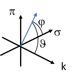
For the magnetic field its field strength and two angles are given. The polar angle \(\vartheta\) is defined from the \(k\) vector. The azimuthal angle \(\varphi\) is defined in the \(\sigma - \pi\) plane from the \(\sigma\) direction.
For a magnetic field along \(k\) (Faraday geometry) set the Hyperfine parameters to
hyperfine = nx.Hyperfine(
   magnetic_field = 33,         # magnetic field in T
   magnetic_theta = 0,          # polar angle
   magnetic_phi = 0)            # azimuthal angle
For a magnetic field along \(\sigma\) set it to
hyperfine = nx.Hyperfine(
   magnetic_field = 33,         # magnetic field in T
   magnetic_theta = 90,         # polar angle
   magnetic_phi = 0)            # azimuthal angle
and for a magnetic field along \(\pi\) to
hyperfine = nx.Hyperfine(
   magnetic_field = 33,         # magnetic field in T
   magnetic_theta = 90,         # polar angle
   magnetic_phi = 90)           # azimuthal angle
A magnetic field can be given in the Nexus frame can be converted to spherical coordinates and vie versa with the functions MagVectorToSpherical() and MagSphericalToVector().
New in version 1.0.2.
# Nexus frame (sigma, pi, k)
# spherical (mag, polar, azimuthal)

# convert a magnetic field along pi direction to spherical coordinates
print(nx.MagVectorToSpherical(0, 33, 0))

# convert a magnetic field along k direction to Nexus frame
print(nx.MagSphericalToVector(33, 0, 0))
(33.0, 90.0, 90.0)

(0.0, 0.0, 33.0)
Electric field gradient
The electric field gradient tensor is defined by the largest principal tensor component \(V_{zz}\), the asymmetry parameter \(\eta\), and three Euler angles. In Nexus, instead of \(V_{zz}\) the quadrupole splitting \(QS\) in mm/s is given. The quadrupole energy is
See also
https://en.wikipedia.org/wiki/Electric_field_gradient
https://en.wikipedia.org/wiki/Quadrupole_splitting
For the energy conversion see https://en.wikipedia.org/wiki/Doppler_effect
The angles are the extrinsic Euler angles in ZYZ convention. The angles are thus defined as rotations around the internal fixed-frame coordinate system of Nexus and not around the EFG coordinate system (as in CONUSS). The convention differs in the meaning of the angles \(\alpha\) and \(\gamma\). They are exchanged in the extrinsic and intrinsic convention.
Note
If you want to use Euler angles as in CONUSS just exchange the values of \(\alpha\) and \(\gamma\) in the definition of Hyperfine.
The angle \(\alpha\) is only needed in case of an asymmetry in the EFG. The ZYZ convention is as follows
rotation around \(\vec{k}\)
rotation around \(\vec{\pi}\),
rotation around \(\vec{k}\).
Without rotation, the EFG main axis \(V_{zz}\) points along \(\vec{k}\). The two components \(V_{xx}\) and \(V_{yy}\) point along \(\sigma\) and \(\pi\), respectively.
As an example we rotate the main axis \(V_{zz}\) to the \(\pi`\) direction. The first rotation is arbitrary as it will rotate \(V_{xx}\) and \(V_{yy}\), which is not important without asymmetry. The second rotation around \(\vec{\pi}\) by 90 degree will rotate \(V_{zz}\) to \(\vec{\sigma}\). The third rotation around \(\vec{k}\) by 90 degree will rotate it to \(\vec{\pi}\).
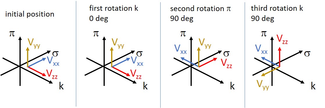
The Euler angles are thus \(\alpha = 0\), \(\beta = \pi/2\) and \(\gamma = \pi/2\). And in Nexus we have
hyperfine = nx.Hyperfine(quadrupole = 0.8,
                         quadrupole_alpha = 0,
                         quadrupole_beta = 90,
                         quadrupole_gamma = 90)
Finding the correct Euler angles by hand can be a tedious task and is prone to error.
Therefore, Nexus provides conversion functions in the euler module.
The same results can be obtained by the functions VectorsToAngles.
If you only want to set the main axis \(V_{zz}\), use
# input vector in the nexus coordinate system [sigma,pi,k]
alpha, beta, gamma = nx.euler.VectorsToAngles([0,1,0])

print(alpha, beta, gamma)  # the return value of alpha is random here
In case you want to set the components \(V_{xx}\) and \(V_{yy}\) as well, use
# input vector in the nexus coordinate system.
# vectors must be orthogonal, but do not have to be normalized
Vzz = [1,0,0]
Vxx = [0,0,1]
Vyy = [0,1,0]
alpha, beta, gamma = nx.euler.VectorsToAngles(Vzz, Vxx, Vyy)

print(alpha, beta, gamma)
In case you have fit some Euler angles, you can also get the EFG vectors by AnglesToVectors.
For more information on Euler angle convention and additional functions have a look to the euler module.
Lamb-Moessbauer factor
New in version 1.1.2.
A site specific Lamb-Moessbauer factor has been added.
If the Material has a :attr:`lamb_moessbauer factor defined, the material`s factor is used.
In case you want to use the site specific Lamb-Moessbauer factor, set the lamb_moessbauer of the Material to None.
In that case each site assigned to the material must have a valid Lamb-Moessbauer factor defined.
Isotropic
The isotropic option sets a 3D angular distribution of the site.
The site parameters (the angels between the magnetic field and the quadrupole) are fixed.
Texture
New in version 1.1.2.
Since version 1.1.2 Nexus offers a texture coefficient as in CONUSS.
It is only used if .isotropic = False.
Please be aware that the texture coefficient relates to a very special situation of hyperfine parameters.
A texture of 1 corresponds to site whose directional parameters are such as given.
A texture of 0 corresponds to a site whose isotropic is set to True.
It means that the non-texture part models a site with BOTH magnetic field and quadrupole slitting randomly distributed in 3D.
All values between 0 and 1 mix the two cases.
Note
Prior to version 1.1.2 use
Texture as in CONUSS
If you are familiar with CONUSS you might want to set the texture of a sample.
Before version 1.1.2, this option was not implemented in Nexus for two reasons:
Users were often not fully aware of the model behind this parameter.
The same result can be obtained with two hyperfine sites. However, with double the computational effort.
The definition via two sites keeps the physical interpretation clearer and the user must exactly know how to set this up.
Here is how to emulate the texture coefficient from CONUSS. Let’s assume a hyperfine site with a magnetic field directed along the photon k-vector. The texture should be 80% in CONUSS. Then, in Nexus write
# this site corresponds to the 80% textured part with both magnetic field and efg
# beeing directed along their given directions
site_1 = nx.Hyperfine(weight = 0.8,
                      magnetic_field = 33,
                      magnetic_theta = 0,
                      magnetic_phi = 0,
                      quadrupole = 0,
                      isotropic = False)

# this site corresponds to the 20% non-textured part with both magnetic field and efg
# being completely spherically distributed
site_2 = nx.Hyperfine(weight = 0.2,
                      magnetic_field = 33,
                      quadrupole = 0,
                      isotropic = True)

material.hyperfine_sites = [site_1, site_2]
When you want to fit a texture just let one of the weights be fitted and keep the other one fixed. As the weight give the relative contribution you can easily calculate the percentage.
Notebooks
hyperfine - nb_hyperfine.ipynb.
Please have a look to the API Reference for more information.