Scattering functions and the refractive index
You can also calculate scattering cross sections, scattering lengths, scattering matrices or refractive indices of elements, materials, layers or samples.
Electronic scattering cross sections
Here, various electronic scattering cross sections calculations are shown. Klein-Nishina scattering is calculated after [KleinNishina]. Photoeffect cross sections are calculated after [Smith]. The electronic cross section is the sum of both contributions.
import nexus as nx

Au = nx.Element(element = "Au")

klein = nx.KleinNishinaCrossSection(Au, 14.4125e3)
print(klein)

photo = nx.PhotoCrossSection(Au, 14.4125e3)
print(photo)

elec = nx.ElectronicCrossSection(Au, 14.4125e3)
print(elec)
the functions return the cross section in \(m^2\).
4.979260700505022e-27
5.847566888130204e-24
5.852546148830709e-24
Scattering Length
The scattering length can be calculated with the cross sections calculated in the previous example or with tabulated values from the CXRO webpage [Henke] and [CXRO].
If the CXRO values are the standard values. If the cross section calculation should be used, use the appropriate set method.
# Change Nexus calculation method for the atomic scattering factors
nx.SetAtomicScatteringFactorCXRO(False)

# Get method
print(nx.GetAtomicScatteringFactorCXRO())
In the following example, the cross section calculation is used.
import nexus as nx
import numpy as np
import matplotlib.pyplot as plt

scat = nx.ElectronicScatteringLength(Au, 14.4125e3, cxro = False)
print(scat)

scat_matrix = nx.ElectronicScatteringLengthMatrix(Au, 14.4125e3, False)
print(scat_matrix)
the functions return the scattering length in \(m\).
(-2.2007448586170272e-13+3.4016359521004525e-14j)
[[-2.20074486e-13+3.40163595e-14j  0.00000000e+00+0.00000000e+00j]
 [ 0.00000000e+00+0.00000000e+00j -2.20074486e-13+3.40163595e-14j]]
To calculate the nuclear scattering length use
detuning  = np.linspace(-100, 100, 5)

Fe = nx.Material.Template(nx.lib.material.Fe)

site = nx.Hyperfine(magnetic_field = 33)

Fe.hyperfine_sites = [site]

nuc_scat = nx.NuclearScatteringLength(Fe, nx.lib.moessbauer.Fe57, detuning)

print(np.squeeze(nuc_scat))
You will get a a list with 2x2 matrices
[[[ 7.83414010e-15+6.65456280e-17j -4.84239721e-17+3.34860264e-15j]
  [ 4.84239721e-17-3.34860264e-15j  7.83414010e-15+6.65456280e-17j]]

 [[-4.03270478e-14+4.75658449e-15j -4.69310792e-15-4.81382836e-14j]
  [ 4.69310792e-15+4.81382836e-14j -4.03270478e-14+4.75658449e-15j]]

 [[-1.02636288e-30+1.05490530e-15j  0.00000000e+00+8.91495773e-15j]
  [ 0.00000000e+00-8.91495773e-15j -1.02636288e-30+1.05490530e-15j]]

 [[ 4.03270478e-14+4.75658449e-15j  4.69310792e-15-4.81382836e-14j]
  [-4.69310792e-15+4.81382836e-14j  4.03270478e-14+4.75658449e-15j]]

 [[-7.83414010e-15+6.65456280e-17j  4.84239721e-17+3.34860264e-15j]
  [-4.84239721e-17-3.34860264e-15j -7.83414010e-15+6.65456280e-17j]]]
Scattering factors, matrices and the refractive index
In order to calculate electronic or nuclear scattering factors, refractive indices or matrices of a material have a look to the Scattering Matrix section.
Here a few examples are given.
Calculation of the refractive index and the pure electronic scattering factor in grazing incidence geometry.
material = nx.Material(id = "my_material",
                       composition = [["Fe", 2], ["O", 3]],
                       density = 5.24)


# refractive index at 20 keV
refractive_index = nx.ElectronicRefractiveIndex(material, 20e3)

print(refractive_index)


# grazing indcidence scattering factor at 20 keV

# k-vector along layer direction at an angle of 0.1 degree
kz = nx.conversions.EnergyToKvectorZ(20e3, 0.1)

scattering_factor = nx.ElectronicGrazingScatteringFactor(material, 20e3, kz)
print(scattering_factor)
(0.9999973883454211+4.5329294878545176e-08j)
(-1516637870.2120943+26323590.339101084j)
Calculation of the total (nuclear + electronic) forward scattering matrix
# scattering matrix at 57-Fe transition energy
mat_Fe = nx.Material.Template(nx.lib.material.Fe_enriched)

site1 = nx.Hyperfine(magnetic_field = 33)

mat_Fe.hyperfine_sites = [site1]

detuning = np.linspace(-100, 100, 5)

scattering_matrix = nx.ForwardScatteringMatrix(mat_Fe, nx.lib.moessbauer.Fe57, detuning)

print(np.squeeze(scattering_matrix))
[[[-4.70744567e+05 +24417.51152663j -3.29906733e+02 +22813.62949622j]
  [ 3.29906733e+02 -22813.62949622j -4.70744567e+05 +24417.51152663j]]

 [[-7.98860983e+05 +56370.18560938j -3.19735833e+04-327960.37172931j]
  [ 3.19735833e+04+327960.37172931j -7.98860983e+05 +56370.18560938j]]

 [[-5.24117627e+05 +31151.08782692j  0.00000000e+00 +60736.54132636j]
  [ 0.00000000e+00 -60736.54132636j -5.24117627e+05 +31151.08782692j]]

 [[-2.49374272e+05 +56370.18560802j  3.19735833e+04-327960.37172931j]
  [-3.19735833e+04+327960.37172931j -2.49374272e+05 +56370.18560802j]]

 [[-5.77490687e+05 +24417.51152392j  3.29906733e+02 +22813.62949622j]
  [-3.29906733e+02 -22813.62949622j -5.77490687e+05 +24417.51152392j]]]
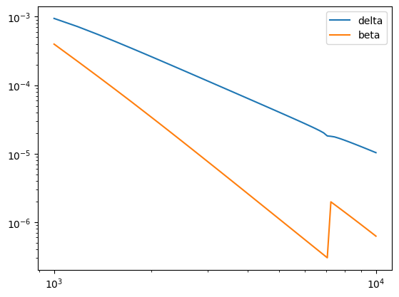
Plotting the refractive index
energies = np.linspace(1000, 10000)
refractive_index = []

for elem in energies:
    refractive_index.append(nx.ElectronicRefractiveIndex(material, elem))

plt.loglog(energies, 1 - np.real(refractive_index), label = "delta")
plt.loglog(energies, np.imag(refractive_index), label = "beta")
plt.legend()
plt.plot()
Scattering parameters of layers and samples
Similar functions exist for Layer and Sample objects. Please have a look to the Layer and Sample sections for a complete list.
For layers and samples, the functions to calculate scattering parameters and so on are class methods.
Calculate refractive index of a layer
import nexus as nx
import nexus as np

layer = nx.Layer(id = "iron oxide layer",
                 thickness = 100,
                 composition = [["Fe", 2], ["O", 3]],
                 density = 5.3)

# at 20 keV
print(layer.ElectronicRefractiveIndex(20e3))
(0.9999973584409794+4.584833260616212e-08j)
Calculate complete grazing incidence layer matrix
mat = nx.Material.Template(nx.lib.material.Fe_enriched)

site = nx.Hyperfine(magnetic_field = 33)

mat.hyperfine_sites = [site]

layer = nx.Layer(id = "my iron oxide layer",
                 thickness = 1000,  # in nanometer
                 material = mat,
                 roughness = 30,
                 thickness_fwhm = 50)

detuning = [0]

matrix = layer.GrazingLayerMatrix(nx.lib.moessbauer.Fe57, detuning, 0.2)

print(np.squeeze(matrix))
The output is a 4x4 matrix for zero detuning only.
[[-4.02131424e+63-3.71188107e+63j -3.71188107e+63+4.02131424e+63j
  -1.36403869e+63+5.83719668e+63j  5.83719668e+63+1.36403869e+63j]
 [ 3.71188107e+63-4.02131424e+63j -4.02131424e+63-3.71188107e+63j
  -5.83719668e+63-1.36403869e+63j -1.36403869e+63+5.83719668e+63j]
 [ 1.36403869e+63-5.83719668e+63j -5.83719668e+63-1.36403869e+63j
  -6.29886297e+63+1.85419632e+63j  1.85419632e+63+6.29886297e+63j]
 [ 5.83719668e+63+1.36403869e+63j  1.36403869e+63-5.83719668e+63j
  -1.85419632e+63-6.29886297e+63j -6.29886297e+63+1.85419632e+63j]]
For a Sample the ObjectMatrix() and the SampleMatrix() are the same.
mat = nx.Material.Template(nx.lib.material.Fe_enriched)

site = nx.Hyperfine(magnetic_field = 33)

mat.hyperfine_sites = [site]

layer = nx.Layer(id = "my iron oxide layer",
                 thickness = 1000,  # in nanometer
                 material = mat,
                 roughness = 30,
                 thickness_fwhm = 50)

sample = nx.Sample(layers = [layer],
                   geometry = "f")

detuning = [0]

matrix = sample.ObjectMatrix(nx.lib.moessbauer.Fe57, detuning, True)
# or
matrix = sample.SampleMatrix(nx.lib.moessbauer.Fe57, detuning)

print(np.squeeze(matrix))
[[-0.69665446+0.67094952j  0.04236449-0.04080134j]
 [-0.04236449+0.04080134j -0.69665446+0.67094952j]]
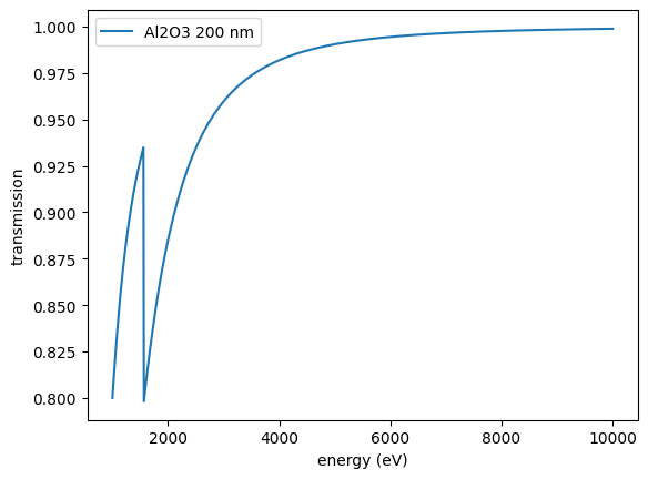
Transmission of a layer / sample
The transmission of a layer can be calculated via
layer = nx.Layer(thickness = 200,
                 material = nx.Material.Template(nx.lib.material.Al2O3))

energies = np.linspace(1000, 10000, 1001)

trans = []

for elem in energies:
    trans.append(layer.ElectronicForwardTransmission(elem))

plt.plot(energies, trans, label = "Al2O3 200 nm")
plt.xlabel("energy (eV)")
plt.ylabel("transmission")
plt.legend()
plt.show()
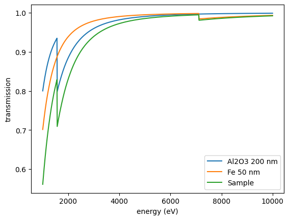
and for a sample via
layer_Al2O3= nx.Layer(thickness = 200,
                 material = nx.Material.Template(nx.lib.material.Al2O3))

layer_Fe = nx.Layer(thickness = 50,
                 material = nx.Material.Template(nx.lib.material.Fe))

sample = nx.Sample(layers = [layer_Al2O3, layer_Fe],
                   geometry = "f")

energies = np.linspace(1000, 10000, 1001)

trans_Al2O3 = []
trans_Fe = []
trans_sample = []

for elem in energies:
    trans_Al2O3.append(layer_Al2O3.ElectronicForwardTransmission(elem))
    trans_Fe.append(layer_Fe.ElectronicForwardTransmission(elem))
    trans_sample.append(sample.ElectronicTransmission(elem))
    # or use trans_sample.append(sample.ElectronicForwardTransmission(elem))

plt.plot(energies, trans_Al2O3, label = "Al2O3 200 nm")
plt.plot(energies, trans_Fe, label = "Fe 50 nm")
plt.plot(energies, trans_sample, label = "Sample")
plt.xlabel("energy (eV)")
plt.ylabel("transmission")
plt.legend()
plt.show()
Please have a look to the API Reference for more information.