Sample
A sample is an object in the beam path. It can consist of several layers and defines the scattering geometry via its position relative to the beam. In grazing-incidence geometry its lateral dimensions and the incoming beam divergence become important.
The following parameters are Var objects and can be fit:
incidence angle of the beam
incoming beam divergence
Scattering geometry
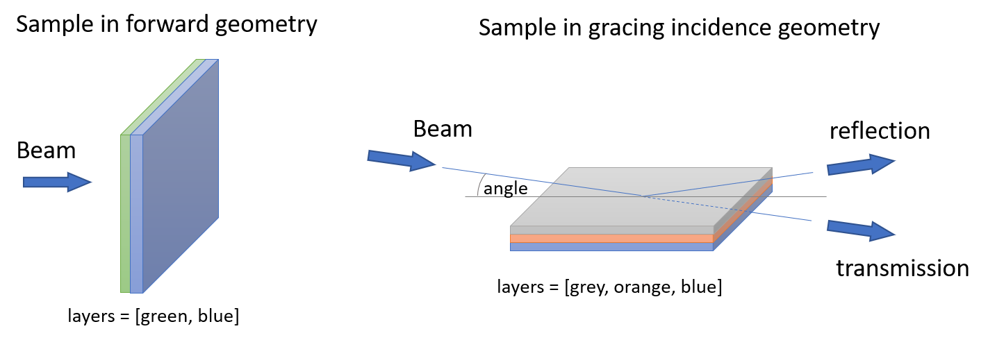
For forward scattering (f) only the layers have to be specified.
In grazing incidence scattering (reflection r or transmission t) the angle, sample length, the roughness model and the incoming beam divergence matter.
import nexus as nx

mat = nx.Material.Template(nx.lib.material.Fe2O3)

site = nx.Hyperfine(magnetic_field = 33,
                    isotropic = True)

mat.hyperfine_sites = [site]

lay = nx.Layer(id = "iron oxide layer",
               thickness = 1000,  # in nanometer
               material = mat,
               roughness = 30,
               thickness_fwhm = 50)

sample = nx.Sample(id = "my sample",
                   layers = [lay],    # list with all layers in beam propagation direction
                   geometry = "f",    # scattering geometry, forward here
                   # the following properties do not matter because of forward geometry
                   # optionally they can be given
                   angle = 0.4,       # incidence angle (degree)
                   length = 10,       # in mm
                   roughness = "a",   # analytical roughness model
                   divergence = 0.0,  # incoming beam divergence (deg)
                   effective_thickness = 0.3,   # nm, only used for effective density model
                   drive_detuning = [],         # Gamma, only used for EnergyTimeSpectra
                   function_time = None)        # time dependent phase factor of a moving sample

print(sample)
The output looks like this
Sample
  .id: my sample
  .geometry: f
  .angle (deg) = 0.4
  .divergence (deg) = 0.0
  .length (mm) = 10.0
  .roughness (model): a
-------|------------------------|---------------|-------------|-------------|--------|-----------|----------|-------------|
 index |               Layer id | dens. (g/cm3) | thick. (nm) | rough. (nm) | abund. | LM factor | HI sites | dist points |
-------|------------------------|---------------|-------------|-------------|--------|-----------|----------|-------------|
     0 |       iron oxide layer |          5.25 |      1000.0 |        30.0 |   0.02 |     0.793 |        1 |           1 |
-------|------------------------|---------------|-------------|-------------|--------|-----------|----------|-------------|
The print outputs a list with all layers in the order along the beam propagation.
Layers
The layers of the sample are given as a list of Layer objects in the order they are passed by the beam.
Layers can be used multiple times in the list.
Typically, you create a Material and Layer object for each layer in the sample. Here, a simple Pt/C/Pt cavity on a silicon substrate is set up.
import nexus as nx
import numpy as np

# layer Pt top #
mat_Pt_top = nx.Material.Template(nx.lib.material.Pt)

lay_Pt_top = nx.Layer(id = "Pt top",
                      material = mat_Pt_top,
                      thickness = 2,
                      roughness = 0.2)


# layer C #
mat_C = nx.Material.Template(nx.lib.material.C)

lay_C = nx.Layer(id = "C",
                 material = mat_C,
                 thickness = 20,
                 roughness = 0.3)

# layer Pt #
mat_Pt = nx.Material.Template(nx.lib.material.Pt)

lay_Pt = nx.Layer(id = "Pt",
                  material = mat_Pt,
                  thickness = 15,
                  roughness = 0.2)

# layer Si #
mat_Si = nx.Material.Template(nx.lib.material.Si)

lay_substrate = nx.Layer(id = "Si sub",
                         material = mat_Si,
                         thickness = nx.inf,
                         roughness = 0.2)

sample = nx.Sample(layers = [lay_Pt_top, lay_C, lay_Pt, lay_substrate],
                   geometry = "r",
                   length = 10,   # mm
                   roughness = "a")
Angle and divergence
The angle is only used in gracing incidence geometry.
It specifies the incidence angle of the photon on the sample measured from the sample surface.
The divergence is specified as the full width half maximum of a Gaussian distribution around the incidence angle.
The divergence distribution is treated incoherently.
This assumption is justified as the transverse coherence length at 3rd generation synchrotrons is typically small.
Note that for the divergence to be taken into account, the distribution_points value of the specific measurement must be larger than 1.
Sample length
The sample length is only used in grazing incidence geometry.
Due to the limited sample size the beam will not completely illuminate the sample at small grazing angles.
Therefore, the reflected intensity is smaller at small angles.
The sample length is the one along the beam propagation direction.
The combination of the beam size Beam.fwhm and the sample length define the portion of the beam that is reflected.
Roughness model
The roughness model is used in gracing incidence geometry only.
It can be analytical (a), no roughness (n), or an effective density model (e).
Please note that the modeling of roughnesses of thin films deserves a whole chapter.
The main problem is that the analytical models are only valid for quite low roughnesses and real films can often exceed this limit.
Nexus will warn you in case the validity is stressed too much. The output will look like this
-------------------------------------------------------------------------------------------
 NEXUS WARNING in Reflectivity
 warning: Analytical roughness model of interface W matrix not valid! Output might be wrong!
          At angle 0.400000 and at energy 14412.497000.
          Wavevector kz * roughness.value = 0.392624 > 0.3 but should be << 1.
          Encountered in Sample.id: simple layers  - Layer.id: Pt  - Layer.roughness: 0.770000
-------------------------------------------------------------------------------------------
Always check for such an error.
Warning
Although the electronic reflectivities often look good even when the roughness is high, never trust a nuclear calculation when you get such an error. For nuclear calculations reduce the layer roughness, introduce interface layers, or use the effective density model to do a proper calculation.
You can use an effective density model to get around this problem.
The layers will be divided in thin slices with the thickness specified by effective_thickness.
These slices are then weighted depending on the roughness specified.
In this way it is even possible to get contributions from several layers to a slice when roughnesses are large.
Note
The effective density model is computational inefficient, especially in nuclear calculations.
Let’s have a look how to work with the effective density model. First we setup three layers on a substrate.
import nexus as nx
import numpy as np
import matplotlib.pyplot as plt

lay_Pt_top = nx.Layer(id = "Pt top",
                      material = nx.Material.Template(nx.lib.material.Pt),
                      thickness = 2,
                      roughness = 0.2)

lay_C = nx.Layer(id = "C",
                 material = nx.Material.Template(nx.lib.material.C),
                 thickness = 20,
                 roughness = 0.3)

lay_Pt = nx.Layer(id = "Pt",
                  material = nx.Material.Template(nx.lib.material.Pt),
                  thickness = 15,
                  roughness = 0.2)

lay_substrate = nx.Layer(id = "Si sub",
                         material = nx.Material.Template(nx.lib.material.Si),
                         thickness = nx.inf,
                         roughness = 0.2)


sample = nx.Sample(layers = [lay_Pt_top, lay_C, lay_Pt, lay_substrate],
                   geometry = "r",
                   length = nx.inf,
                   roughness = "a")
The sample length is set to infinity in order not to have any beam footprint effects. Set up the experiment and the reflectivity.
beam  = nx.Beam()

exp = nx.Experiment(beam = beam,
                    objects = [sample],
                    isotope = nx.moessbauer.Fe57,
                    id = "my exp")

angles = np.arange(0.001, 2, 0.0001, dtype = np.double)

reflectivity = nx.Reflectivity(experiment = exp,
                               sample = sample,
                               energy = nx.lib.energy.CuKalpha,
                               angles = angles)

refl_a = reflectivity()

plt.semilogy(angles, refl_a)
plt.xlabel('angle (deg)')
plt.ylabel('reflectivity')
plt.show()
You will get the following warning and a graph
NEXUS WARNING in Reflectivity
warning: Analytical roughness model of interface W matrix not valid! Output might be wrong!
         At angle 1.999900 and at energy 8047.800000.
         Wavevector kz * roughness.value = 0.426982 > 0.3 but should be << 1.
         Encountered in Sample.id:   - Layer.id: C  - Layer.roughness: 0.300000
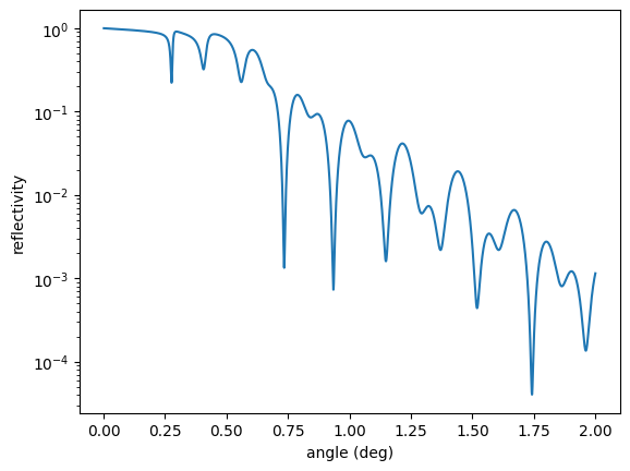
The combination of energy, angle, and roughness makes the analytical model questionable. Let’s calculate without roughness and with the effective density model
sample.roughness = "n"
refl_n = reflectivity()

sample.roughness = "e"
refl_e = reflectivity()

plt.semilogy(angles, refl_a, label = "analytical")
plt.semilogy(angles, refl_n, label = "none")
plt.semilogy(angles, refl_e, label = "effective")

plt.legend()
plt.xlabel('angle (deg)')
plt.ylabel('reflectivity')
plt.show()
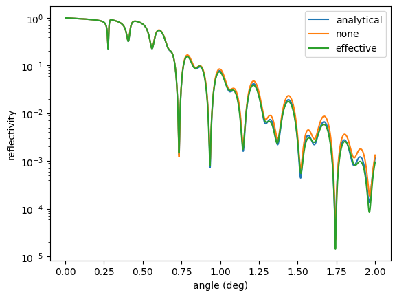
The analytical and effective model are quite similar. Let’s increase the roughness of one layer and recalculate
lay_C.roughness = 3.0

sample.roughness = "a"
refl_a = reflectivity()

sample.roughness = "n"
refl_n = reflectivity()

sample.roughness = "e"
refl_e = reflectivity()

plt.semilogy(angles, refl_a, label = "analytical")
plt.semilogy(angles, refl_n, label = "none")
plt.semilogy(angles, refl_e, label = "effective")

plt.legend()
plt.xlabel('angle (deg)')
plt.ylabel('reflectivity')
plt.show()
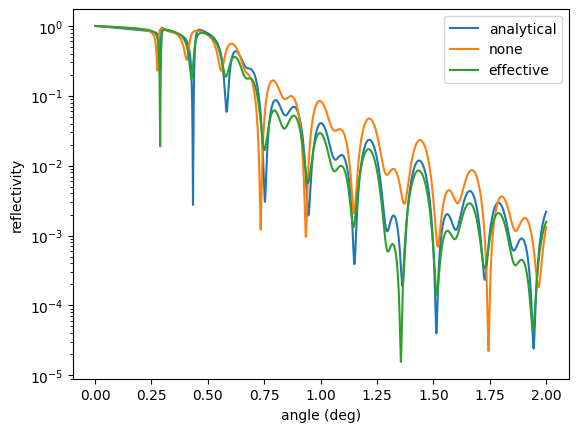
The analytical and effective density models deviate because of the high roughness, which is not properly handled by the analytical assumptions. Keep in mind that the effective density model is also just an approximation. But the best we can do here for higher roughnesses. For more information on the effective density model see Effective density model.
Drive detuning
The drive detuning is a special attribute only used for the EnergyTimeSpectrum measurement class.
It is a list of detuning values which are used to detune the sample in energy with respect to other objects in the beam path.
In the experiment it is done by a Moessbauer drive.
The detuning will change the interference of the different objects.
In this way detuning resolved time spectra can be obtained, which form the EnergyTimeSpectrum object.
There are several methods to retrieve the scattering matrix, refractive index and so forth of a sample. Please have a look to the Sample API for more information.
Air
A special function exists that creates a Sample type of air with a given length.
import nexus as nx

# air of 1 meter
air = nx.Air(1)

print(air)

beam = nx.Beam()
beam.LinearSigma()

exp = nx.Experiment(beam = beam,
                    objects = [air])

intensities = nx.Intensities(experiment = exp,
                             energy = 14400)

print(intensities())
Moving Sample
New in version 1.0.4.
The function_time describes a sample motion along the beam direction.
The time scales are typically on the order of the isotope lifetime as realized with piezo transducers.
The function_time is implemented by the FunctionTime class.
The user can define arbitrary motions of the sample.
The function must return the phase factor \(\phi(t) = k x(t)\),
where \(k\) is the photon wave vector along beam direction and \(x(t)\) the sample motion along the beam propagation direction.
See Time dependence.
Simple sample
New in version 1.0.4.
A new SimpleSample class is available.
It creates a Sample with only one layer and material.
All needed instances are created automatically.
The layer and material parameters can be assigned directly via the SimpleSample attributes.
The code
import nexus as nx

site = nx.Hyperfine(magnetic_field = 33,
                    isotropic = True)

sample = nx.SimpleSample(thickness=3000,
                       composition = [["Fe", 1]],
                       density = nx.Var(7.874, min=7, max=7.874, fit=True, id = "sample density"),
                       isotope = nx.lib.moessbauer.Fe57,
                       abundance = 0.02119,
                       lamb_moessbauer = 0.796,
                       hyperfine_sites = [site])

print("\nthickness change")

print(sample.thickness)

sample.thickness = 1000

print(sample.thickness)


print("\ndensity change of the sample material")

sample.density = 7.3

print(sample.material)

print("\nlayer")

print(sample.layer)


print("\nchange hyperfine sites")

print(list(sample.hyperfine_sites))

site2 = nx.Hyperfine(magnetic_field = 20,
                     isotropic = True)

sample.hyperfine_sites = [site,site2]

print("new hyperfine sites")

print(list(sample.hyperfine_sites))
will give the output
thickness change
Var.value = 3000.0, .min = 0.0, .max = inf, .fit: False, .id:
Var.value = 1000.0, .min = 0.0, .max = inf, .fit: False, .id:

density change of the sample material
Material
  .id:
  .composition:  Fe 1.0
  .density (g/cm^3) Var.value = 7.3, .min = 7.0, .max = 7.874, .fit: True, .id: sample density
  .isotope: 57-Fe
  .abundance Var.value = 0.02119, .min = 0.0, .max = 1.0, .fit: False, .id:
  .lamb_moessbauer Var.value = 0.796, .min = 0.0, .max = 1.0, .fit: False, .id:
    derived parameters:
    .total_number_density (1/m^3) = 7.868823760260314e+28
    .average_mole_mass (g/mole) = 55.868105434026994
    .isotope_number_density (1/m^3) = 1.6674037547991608e+27
    number of hyperfine sites 1


layer
Layer
  .id:
  .material.id:
  .material.composition:  Fe 1.0,
  .material.density (g/cm^3) Var.value = 7.3, .min = 7.0, .max = 7.874, .fit: True, .id: sample density
  .thickness (nm) Var.value = 1000.0, .min = 0.0, .max = inf, .fit: False, .id:
  .roughness (nm, sigma) Var.value = 0.0, .min = 0.0, .max = inf, .fit: False, .id:
  .thickness_fwhm (nm) Var.value = 0.0, .min = 0.0, .max = inf, .fit: False, .id:


change hyperfine sites
[Hyperfine .id:
  .weight =               1.0
  .isomer_shift =         0.0        dist points: 1
  .magnetic_field =       33.0       dist points: 1
  .magnetic_theta =       0.0        dist points: 1
  .magnetic_phi =         0.0        dist points: 1
  .quadrupole =           0.0        dist points: 1
  .quadrupole_alpha =     0.0        dist points: 1
  .quadrupole_beta =      0.0        dist points: 1
  .quadrupole_gamma =     0.0        dist points: 1
  .quadrupole_asymmetry = 0.0        dist points: 1
  .isotropic =            True       3D distribution in mag and efg. Random mag or efg distributions are ignored.
  random magnetic distribution: none         dist points: 1
  random quadrupole distribution: none       dist points: 1
  total number of distribution points: 1
]
new hyperfine sites
[Hyperfine .id:
  .weight =               1.0
  .isomer_shift =         0.0        dist points: 1
  .magnetic_field =       33.0       dist points: 1
  .magnetic_theta =       0.0        dist points: 1
  .magnetic_phi =         0.0        dist points: 1
  .quadrupole =           0.0        dist points: 1
  .quadrupole_alpha =     0.0        dist points: 1
  .quadrupole_beta =      0.0        dist points: 1
  .quadrupole_gamma =     0.0        dist points: 1
  .quadrupole_asymmetry = 0.0        dist points: 1
  .isotropic =            True       3D distribution in mag and efg. Random mag or efg distributions are ignored.
  random magnetic distribution: none         dist points: 1
  random quadrupole distribution: none       dist points: 1
  total number of distribution points: 1
, Hyperfine .id:
  .weight =               1.0
  .isomer_shift =         0.0        dist points: 1
  .magnetic_field =       20.0       dist points: 1
  .magnetic_theta =       0.0        dist points: 1
  .magnetic_phi =         0.0        dist points: 1
  .quadrupole =           0.0        dist points: 1
  .quadrupole_alpha =     0.0        dist points: 1
  .quadrupole_beta =      0.0        dist points: 1
  .quadrupole_gamma =     0.0        dist points: 1
  .quadrupole_asymmetry = 0.0        dist points: 1
  .isotropic =            True       3D distribution in mag and efg. Random mag or efg distributions are ignored.
  random magnetic distribution: none         dist points: 1
  random quadrupole distribution: none       dist points: 1
  total number of distribution points: 1
]