Fitting and Optimization
Nexus offers the non-linear optimization modules Fit and Optimizer.
Fitting theoretical models to experimental data is only one problem encountered in non-linear optimization.
In general, the goal is to find a local minimum or maximum of a problem.
In Nexus, this minimization procedure can also be used to design experiments to specific target values.
Nexus will always minimize a least squares problem.
The Fit module is intended to fit single or multiple data sets.
The fitting routines are not limited to the same Experiment but arbitrary combinations of experiments, samples, measurements and so on can be fit in a consistent way.
The Fit method can only be applied to FitMeasurement types, like a reflectivity or a time spectrum for example.
The Optimizer module is used to optimize an experiment to specific design parameters.
The user can define arbitrary target functions (residuals) to be minimized and which depend on Vars.
The Optimizer will then minimize your target function.
It is intended for theoretical calculations and can be applied to all Measurement types.
There are different non-linear optimization algorithms implemented in Nexus. The algorithms tackle your problem in different ways in order to find the best solution to your problem. They can be divided in local and global algorithms.
Local optimization should be used when you do not expect various local minima in the search area or the initial guess is already close to the global minima. The local methods can be further divided in gradient-based and gradient free methods.
Global optimization should be used when you do not know much about your problem or you expect various local minima in the search region.
After a global optimization Nexus will call a local method. This is done in order to find the local minimum around the minimum of the global method.
One of the most prominent algorithm is the Levenberg-Marquardt algorithm LevMar, a gradient-based local algorithm. This one is typically the first one to use.
In global optimization the Differential Evolution algorithm is very powerful and PagmoDiffEvol is typically your first choice.
A full list of all algorithms can be found here, OptimizerOptions.
See also
https://en.wikipedia.org/wiki/Levenberg-Marquardt_algorithm
https://en.wikipedia.org/wiki/Differential_evolution
http://ceres-solver.org/nnls_tutorial.html
The residual in data fitting
Both modules try to minimize the residual
of each data point, where \(y\) is the experimental or target value and \(y^t\) is the theoretical value of your model. From the residuals Nexus calculates a \(cost\) function which is the target value to be minimized
It is half the value of the chi-squared function.
In data fitting this residual often has to be weighted properly by the error of the measured point. A commonly used weighted residual in least square fitting is
where \(y_i\) is a measured data point and \(y^t_i\) is the corresponding theoretical model value. This will result in the \(cost\) function
It is the best unbiased estimator for uncorrelated errors.
However, for the count statistics typically encountered in reflectivity or NRS measurements a better estimator can be found.
In Nexus the default residual for fitting is
Changed in version 1.0.3: For the classes Reflectivity and Transmission a log norm is applied now as the standard residual \(r_i = \log_{10}(y_i) - \log_{10}(y^t_i)\).
with the \(cost\) function
\[cost = \frac{1}{2} \sum_i \left(\sqrt{y_i} - \sqrt{y^t_i}\right)^2\]
It is an approximation of a Poisson likelihood function [Thibault], which is better suited for Poisson statistics (low counts) as often encountered in time spectra and reflectivities. The residual is always internally squared by the fitting and optimization routines in Nexus to fit a least squares problem. Therefore, the log likelihood estimator is not directly implementable. At larger count numbers the Poisson statistics approach a Gaussian distribution. For Gaussian statistics, the likelihood function corresponds to the weighting with the standard deviation [Thibault]. Therefore, the difference between both estimators is typically small.
The residual implementation used in fitting can be changed by the Residual class, Residual.
For example, to use the weighting by the standard deviation use nx.residual.StdDev.
More residual implementations can be found in residual.
The residual in optimization problems
For an optimization problem the residual is the difference between your target value and the model output.
Let’s have a look at a simple example.
You want to minimize the intensity \(I\) behind a sample that depends on various Var objects \(v_i\).
The target value is \(0\) as the intensity should be minimal and cannot be negative.
The corresponding residual is
The minimization procedure will try to minimize the squared residual, which is the squared intensity in this case.
Especially in fitting and optimization the class referencing strategy of Python and Nexus gets very important.
Please remember the sections Introduction and Multilayers and Nexus references where referencing in Nexus is explained.
If different objects reference the same Var object, its value is used for all referencing objects.
This allows to couple a single Var to various objects while fitting.
For multi measurement fits, referencing can get very important, for example, when the same Sample or one of its properties has to be referenced in different Experiments and Measurements.
Fitting
The Fit module fits the theoretical model parameters to experimental data sets.
In order to do so, the intensity and the corresponding free parameter (detuning, time, angle, …) have to be specified in the FitMeasurements.
The fit module only takes a list of FitMeasurement objects as an argument.
As all the corresponding model parameters are defined in the Experiment and the experimental data and conditions are defined in the FitMeasurement, the latter is the only object needed to perform the fit.
The module will find every Var object it depends on and automatically adds them to the fit.
Remember that every fit parameter has to be defined as a Var whose fit attribute is set to True.
Vars that are set to .fit = True but do not belong to the one of the passed measurements will not be taken into account.
A FitMeasurement object has a scaling which is always added to the fit even if not defined as a fit parameter.
This behavior can be changed by defining the scaling as a Var and setting .fit = False.
You should always define reasonable min and max boundaries for a fit variable.
For the gradient-based local algorithms that is often not needed to run a good fit but for global methods it is mandatory.
Otherwise the search areas can be totally unrealistic and the fit might never find a good minimum.
Go to the Hello Nexus for a basic fit example. It used the Levenberg-Marquardt and the Differential Evolution algorithm. We will repeat this example here but use another global fit algorithm.
Fit options
All options of the fit module are accessible by the options attribute.
It is an instance of the OptimizerOptions class.
To change the algorithm, for example, you can create a fit object and change the algorithm like this
import nexus as nx

fit = nx.Fit(id = "my fit module")

fit.options.method = "DiffEvol"
# or
fit.options.method = "BeeColony"
# or
fit.options.method = "BasinHopping"

# or you can change the maximum number of iterations of the fit module
fit.options.iterations = 100
There are a lot of options in the OptimizerOptions.
Four methods have special options, those are the LineSearch, CompassSearch, DiffEvol, and BasinHopping.
In case you want to change parameter of these use
# set the inner algorithm of the Basin Hopping method
fit.options.BasinHopping.inner = "Compass"

# or set the number of unsuccessful iterations
fit.options.BasinHopping.stop = 10
Please have a look at the OptimizerOptions for all options of both Fit and Optimizer module.
Global fitting
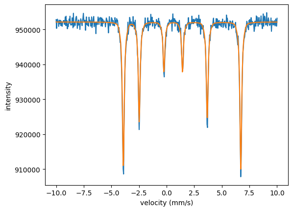
Here, an example similar to the one the Hello Nexus example is treated but with the global fitting algorithm BasinHopping.
Note
Always define reasonable boundaries on a fit variable for global optimization.
This also holds for the scaling parameter of a FitMeasurement method.
The auto option for scaling or background will set boundaries but with a quite large range.
import nexus as nx
import numpy as np
import matplotlib.pyplot as plt
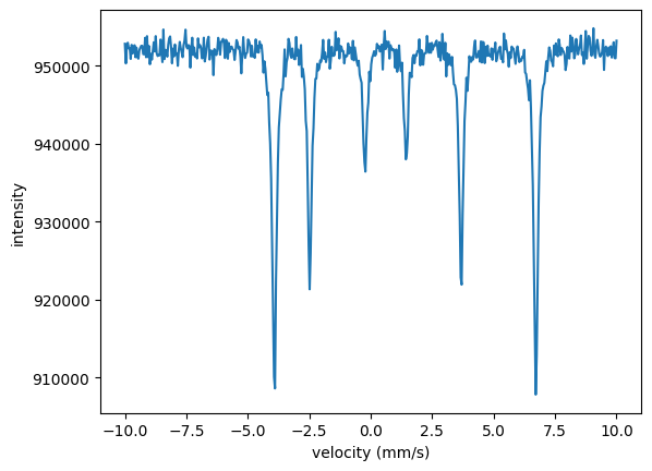
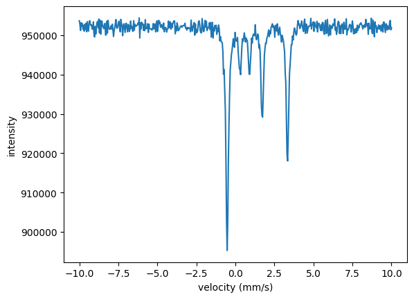
velocity_experiment, intensity_experiment = nx.data.Load('example_spectrum.txt', 0, 1)
site = nx.Hyperfine(magnetic_field = nx.Var(value = 28, min = 25, max = 35, fit = True, id = "magnetic field"),
isotropic = True)
mat_Fe = nx.Material.Template(nx.lib.material.Fe)
mat_Fe.hyperfine_sites = [site]
layer_Fe = nx.Layer(id = "Fe",
material = mat_Fe,
thickness = 3000)
sample = nx.Sample(layers = [layer_Fe])
beam = nx.Beam()
beam.Unpolarized()
exp = nx.Experiment(beam = beam,
objects = [sample],
isotope = nx.lib.moessbauer.Fe57)
spectrum = nx.MoessbauerSpectrum(experiment = exp,
velocity = velocity_experiment,
intensity_data = intensity_experiment,
scaling = "auto")
# calculate the intensity from the assumed model
intensity = spectrum.Calculate()
# plot both the model and the measured data
plt.plot(velocity_experiment, intensity_experiment)
plt.plot(velocity_experiment, intensity)
plt.xlabel('velocity (mm/s)')
plt.ylabel('intensity')
plt.show()
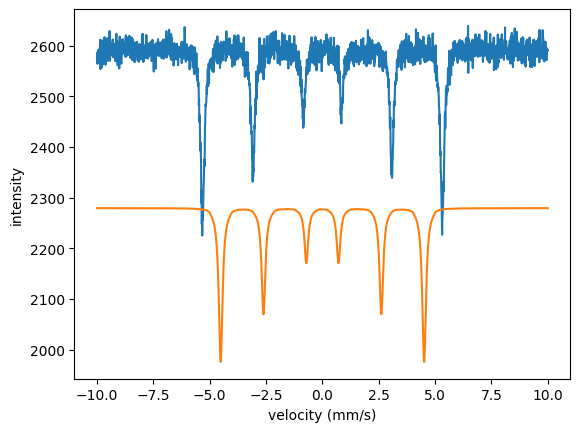
Both the scaling and the hyperfine field are off. Now run the fit.
# create a fit object with a list of measurements to be fit in parallel.
fit = nx.Fit(measurements = [spectrum])
# change to the basin hopping algorithm with inner algorithm suplex
fit.options.method = "BasinHopping"
fit.options.BasinHopping.inner = "Subplex"
# run the fit
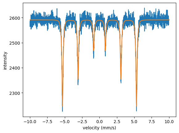
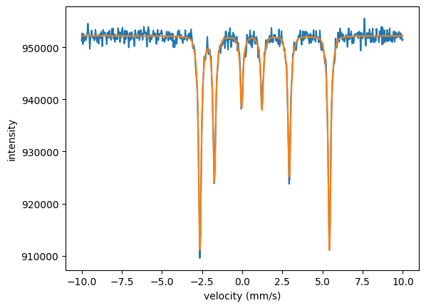
fit.Evaluate()
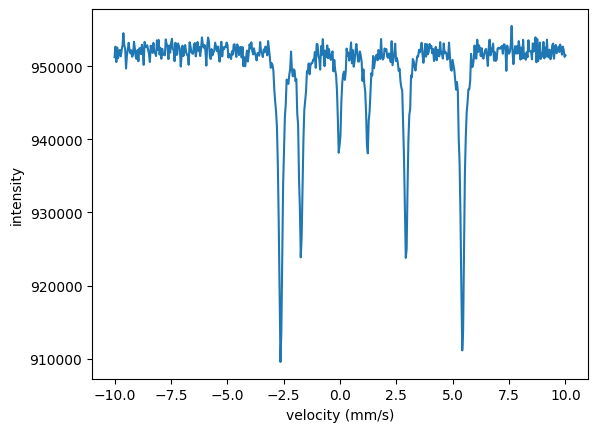
plt.plot(velocity_experiment, intensity_experiment)
plt.plot(velocity_experiment, spectrum.result)
plt.xlabel('velocity (mm/s)')
plt.ylabel('intensity')
plt.show()
The fit object will give the following output
Starting fit with 1 measurement data set(s) and 2 fit parameter(s).

  no. |                           id |       initial value |              min |              max
    0 |                   ES scaling |             2638.74 |                0 |           263874
    1 |               magnetic field |                  28 |               25 |               35

Calling Pagmo solver with fit method BasinHopping

inner algorithm: Subplex
  population: 30
  iterations: 100

  cost = 2.136686e+01

Calling ceres solver with fit method LevMar

Ceres Solver Report: Iterations: 1, Initial cost: 2.136686e+01, Final cost: 2.136686e+01, Termination: CONVERGENCE

Fit performed with 2 fit parameter(s).

  no. |                           id |           fit value |       initial value |              min |              max
    0 |                   ES scaling |             3000.47 |             2638.74 |                0 |           263874
    1 |               magnetic field |             32.9955 |                  28 |               25 |               35

  total cost = 2.136686e+01

cost for each FitMeasurement is:

  no. |                           id |                cost |                   %
    0 |                              |        2.136686e+01 |             100.000
You can observe that the global fit algorithm BassinHopping is followed by a call of the local algorithm LevMar.
This is the local search following the global optimization.
In case you want to change the algorithm of the local search you can change it with the options.local attribute.
Let’s have a look to the fit result.
In case you want to set the fit parameters back to their initial values use the SetInitialVars() method
fit.SetInitialVars()

plt.plot(velocity_experiment, intensity_experiment)
plt.plot(velocity_experiment, spectrum())
plt.xlabel('velocity (mm/s)')
plt.ylabel('intensity')
plt.show()

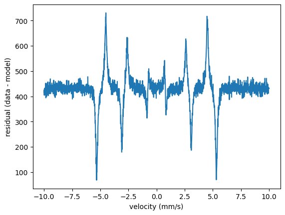
In order to look how the residuals are distributed (now with the initial parameters again) just do
residuals = intensity_experiment - spectrum()

plt.plot(velocity_experiment, residuals)
plt.ylabel('residual (data - model)')
plt.show()
Residuals
The residual is the difference of the experimental value and the theoretical value
However, in fitting this residual has to be weighted properly in order to account for the underlying measurement statistics.
Nexus uses the cost function
This is the default residual weight function in Nexus if no residual of a measurement is specified (None) or if nx.lib.residual.Sqrt() is used, see residual section.
Note
For the classes Reflectivity and Transmission a log norm is applied now as the standard residual \(r_i = \log_{10}(y_i) - \log_{10}(y^t_i)\).
Changed in version 1.0.3.
The Python implementations enable you to change the residual calculation to your needs.
In case you want to change the residual you can take the ones from the lib.residual library (residual).
For example, you can change the residual not to be weighted just by specifying the difference of the values
reflectivity = nx.Reflectivity(experiment = ...,
                               sample = ...,
                               energy = ...,
                               angles = ...,
                               intensity = ...,
                               residual = nx.lib.residual.Difference()
                               scaling = ...,
                               ...)
It is also possible to define your own residual weighting using the Residual class.
Let’s implement a square root scaling.
This already exits as nx.lib.residual.Sqrt but it will serve as as an example.
class MySqrt(nx.Residual):
    # standard initializer
    def __init__(self, id = "MySqrt"):
        super().__init__(id)

    # residual function implementation
    # keep the inputs as they are
    def ResidualFunction(self, input_data, input_theory):
        sqrt_data = np.where(np.array(input_data) >= 0, np.sqrt(input_data), 0.0)
        sqrt_theory = np.where(np.array(input_theory) >= 0, np.sqrt(input_theory), 0.0)
        return np.subtract(sqrt_data, sqrt_theory)

 # pass your implementation
 reflectivity.residual = MySqrt()
That’s it.
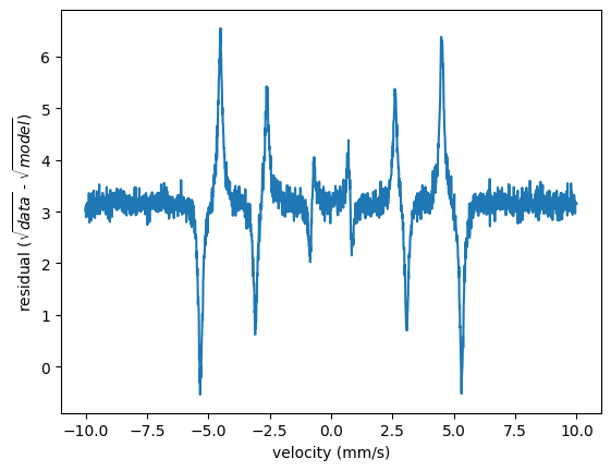
In order to look for the weighted residuals of the global fit example given before you can do
residuals = nx.lib.residual.Sqrt().ResidualFunction(intensity_experiment, spectrum.result)

plt.plot(velocity_experiment, residuals)
plt.xlabel('velocity (mm/s)')
plt.ylabel('residual ($\sqrt{data}$ - $\sqrt{model}$)')
plt.show()
Note
Be careful not to run into any division by zero or any kind of similar problem in your own implementation.
Error estimation
New in version 1.1.0.
Nexus provides tools for error analysis on the fit parameters. Two methods for error calculations are provided. The first one is based on the gradient-based local search algorithms of the ceres solver. The second method is based on a resampling strategy called bootstrapping.
Always keep in mind that reliable error analysis of fit problems is a complicated task. The calculated errors are the estimated standard deviations of the fit parameter.
Gradient based error analysis
For this model to be valid, a normal distribution of the errors with zero mean is assumed.
The error calculation is based on the gradient approach using the Jacobian matrix \(J\) of the fit problem. The inverse Hessian matrix is
or in the case of a rank-deficient \(J\) (meaning some parameters have no influence on the fit problem), \(H\) is given by the Moore-Penrose pseudo inverse
The fit problem will generate a covariance matrix \(C\) describing the joint variability of the fit parameters. The covariance matrix is
with
where \(w_i\) is the weight of the residual, \(r_i\) is the residual implementation, \(n_d\) is the number of data points of the fit problem, and \(n_p\) is the number of fit parameters.
Bootstrap error analysis
Bootstrapping is a random resampling technique to estimate the variability of a fit parameter from a single data set. The newly generated data sets are fit and from all the fits the mean fit parameters, errors and the covariance matrix are determined. A typical number of bootstrap data sets is between 50 to 100. So, the method is computationally expensive. The benefit is that the underlying distribution function of the data do not need to be known.
Several version exist how to implement the bootstrap algorithm. The main difference is parametric and non-parametric bootstrapping:
Parametric bootstrapping resamples from a known distribution, you trust the underlying model you assume. In Nexus this can be either the Poisson distribution or Gaussian distribution (whose sigma is given by the square root of the variance). A Poisson distribution accounts for the proper count statistics of a histogram.
Non-parametric bootstrapping does not make any assumption on the underlying distribution function. The data points have to be resampled without using any model assumption on the data. Therefore, residual bootstrapping, wild bootstrapping, and smooth bootstrapping are used. The residual bootstrap takes the first fit and randomly picks a residual (from all the residuals in a data set ) and puts it on the fit curve to generate new bootstrap data sets. Wild bootstrap reweights the residuals of the first fit by a Gaussian distribution with variance one to generate bootstrap data sets. Smooth bootstrapping uses the original data sets and applies a smoothing method (uniform or Gaussian) with smoothing parameter specified by the user. The default is the wild bootstrip as it relies only on the residual of the individual data points and can be apllied to heteroscedastic data sets.
Parameter errors, covariances and the correlation matrix
The covariance measures the joint variability of fit parameters. Both error methods will provide the covariance. The higher the covarinace of two parameters the higher the error of these parameters will be.
The correlation matrix is determined from the Pearson correlation coefficient and measures the linear correlation between two fit parameters. It normalizes the covariance matrix between -1 and 1.
See also
https://en.wikipedia.org/wiki/Correlation
https://en.wikipedia.org/wiki/Pearson_correlation_coefficient
The diagonal elements of the covariance matrix are the variances of the fit parameters and the standard deviation is given by square root of these elements. So the error vector of the estimated standard deviations is
As noted these errors are estimates, especially when the provided residual is not simply weighted by unity or the variance but other functional dependencies are present like the residual.Sqrt or residual.Log10.
Example
Here is an example on how to use the error analysis
import nexus as nx
import numpy as np
import matplotlib.pyplot as plt

data = np.loadtxt('example_spectrum.txt')

velocity_experiment = data[:,0]
intensity_experiment = data[:,1]

site = nx.Hyperfine(isomer = nx.Var(value = 2, min = -3, max = 3, fit = True, id = "isomer"),
                    magnetic_field = nx.Var(value = 31, min = 25, max = 35, fit = True, id = "magnetic field"),
                    magnetic_theta = nx.Var(value = 0, min = -15, max = 15, fit = True, id = "magnetic theta"),
                    quadrupole = nx.Var(value = 0.3, min = 0, max = 2, fit = True, id = "quadrupole"),
                    isotropic = True)

mat_Fe = nx.Material.Template(nx.lib.material.Fe)

mat_Fe.hyperfine_sites = [site]

layer_Fe = nx.Layer(id = "Fe",
                    material = mat_Fe,
                    thickness = nx.Var(value = 2900, min = 0, max = 5000, fit = True, id = "thickness"))

sample = nx.Sample(layers = [layer_Fe])

beam = nx.Beam()

beam.Unpolarized()

exp = nx.Experiment(beam = beam,
                    objects = [sample],
                    isotope = nx.lib.moessbauer.Fe57)

spectrum = nx.MoessbauerSpectrum(experiment = exp,
                                 velocity = velocity_experiment,
                                 intensity_data = intensity_experiment,
                                 scaling = "auto")

intensity = spectrum.Calculate()

fit = nx.Fit(measurements = [spectrum])

# default
# standard call since version 1.1.0
fit.options.error_method = "Gradient"

fit.Evaluate()
Part of the output is
Fit performed with algorithm:
LevMar
Error analysis:
Gradient

Using 6 fit parameter(s):

  no. |                           id |          fit value |   +/- std dev | initial value |          min |          max
    0 |                   ES scaling |            1682.71 |       284.377 |       2638.74 |            0 |       263874
    1 |                    ES backgr |            1276.44 |       308.362 |       257.138 |            0 |      25713.8
    2 |                    thickness |               5000 |       1326.82 |          2900 |            0 |         5000
    3 |               magnetic field |            32.9954 |     0.0095092 |            31 |           25 |           35
    4 |               magnetic theta |                  0 |             0 |             0 |          -15 |           15
    5 |                   quadrupole |        0.000658927 |    0.00259623 |           0.3 |            0 |            2

Correlation matrix:

  no. |        0        1        2        3        4        5
 -----|------------------------------------------------------
    0 |    1.000   -1.000   -0.998   -0.000      nan   -0.000
    1 |   -1.000    1.000    0.999    0.000      nan    0.000
    2 |   -0.998    0.999    1.000    0.000      nan    0.000
    3 |   -0.000    0.000    0.000    1.000      nan    0.000
    4 |      nan      nan      nan      nan      nan      nan
    5 |   -0.000    0.000    0.000    0.000      nan    1.000

Found 1 parameters without influence on the fit model:

  no. |                           id
    4 |               magnetic theta

It is recommended to remove these parameters from the fit or to change the start parameters.
The first three parameters show a strong covariance, meaning that their fit values strongly depend on each other.
This leads to a rather high error (+/- std dev) in these parameters.
The magnetic field and the quadrupole splitting show no correlation to the other parameters ad their errors are rather small.
The polar magnetic angle does not show any influence on the fit.
Its variance is nan.
Such parameters should be removed from the fit or other start parameters should be used.
In order to get the values used for the calculations you can use
inverseHessian = fit.inverse_hessian

covariance_matrix = fit.covariance_matrix

correlation_matrix = fit.correlation_matrix

errors = np.squeeze(fit.fit_parameter_errors)

print(errors)
[2.84377442e+02 3.08362357e+02 1.32681916e+03 9.50919595e-03
 0.00000000e+00 2.59623390e-03]
Scaling and background
The scaling option is set to auto and background option to 0 in the standard setting.
background can also be set to auto in case a background should be fit.
In case you want to set your own values you can change these two attributes
spectrum = nx.MoessbauerSpectrum(experiment = exp,
                                 velocity = velocity_experiment,
                                 intensity_data = intensity_experiment,
                                 scaling = 10,    # constant value
                                 background = "auto")

# or
spectrum = nx.MoessbauerSpectrum(experiment = exp,
                                 velocity = velocity_experiment,
                                 intensity_data = intensity_experiment,
                                 scaling = nx.Var(10, min = 0, max = 100, fit = True, id = "scaling"))

spectrum.background = nx.Var(3, min = 0, max = 20, fit = True, id = "background")
Multi measurement fitting
One of the big advantages of Nexus compared to other software packages is the capability to fit multiple data sets together and even directly fit them to an underlying model.
In order to do so, you just have to provide several FitMeasurements.
The measurements do not need to come from the same Experiment.
You are free in passing any kind of combination of FitMeasurments or models to the fit routines.
Multi-fit from a single experiment
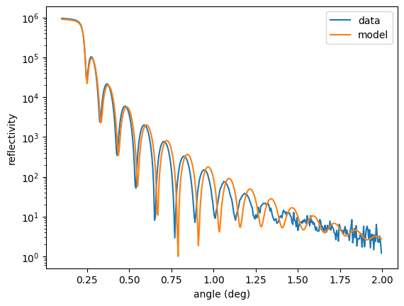
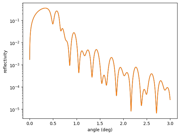
Let’s assume you have several data sets from a single sample, here, an iron thin film on a silicon substrate. The data set consists of a reflectivity and a time spectrum measured at the critical angle (0.225 deg). One could try to fit all data sets one after another, which is often a good idea. You could first get the structural parameters from the reflectivities and the hyperfine parameters from the time spectrum.
Another approach is to fit all data sets together. This can be very helpful when no consistent picture can be found with several single fits or when you have a lot of free parameters in your experiment. Here’s an example how to fit all data together
Load the data.
import nexus as nx
import numpy as np
import matplotlib.pyplot as plt
from scipy.signal import argrelextrema

angles_data, reflectivity_data = nx.data.Load("reflectivity.txt", 0, 1)

time_data, time_spec_data = nx.data.Load("time_spectrum.txt", 0, 1)
Then set up the model and plot all together with initial guesses for some fit parameters.
beam = nx.Beam()
beam.LinearSigma()
# set up Fe layer on Silicon wafer
site = nx.Hyperfine(magnetic_field = nx.Var(32, min = 30, max = 35, fit = True, id = "magnetic field"))
site.SetRandomDistribution(target = "mag", type = "2Dsp", points = 401)
mat_Fe = nx.Material.Template(nx.lib.material.Fe)
mat_Fe.density = nx.Var(7.4, min = 7, max = 7.874, fit = True, id = "Fe density")
mat_Fe.hyperfine_sites = [site]
layer_Fe = nx.Layer(thickness = nx.Var(19.5, min = 17, max = 23, fit = True, id = "Fe thickness"),
roughness = nx.Var(0.5, min = 0.1, max = 1, fit = True, id = "Fe roughness"),
material = mat_Fe)
substrate = nx.Layer(thickness = nx.inf,
roughness = nx.Var(0.1, min = 0.0, max = 1, fit = True, id = "Si roughness"),
material = nx.Material.Template(nx.lib.material.Si))
sample = nx.Sample(layers = [layer_Fe, substrate],
geometry = "r",
length = 10,
roughness = "a")
# experiment
exp = nx.Experiment(beam = beam,
objects = [sample],
isotope = nx.lib.moessbauer.Fe57)
# reflectivity
ref = nx.Reflectivity(experiment = exp,
sample = sample,
energy = nx.lib.energy.Fe57,
angles = angles_data,
intensity_data = reflectivity_data,
resolution = 0.001,
id = "reflectivity")
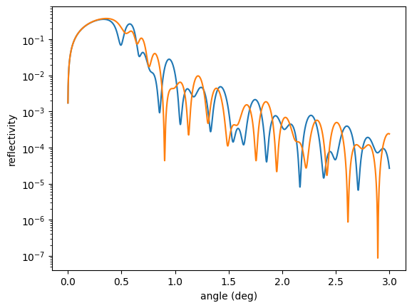
plt.semilogy(angles_data, reflectivity_data, label = "data")
plt.semilogy(angles_data, ref(), label = "model")
plt.legend()
plt.xlabel('angle (deg)')
plt.ylabel('reflectivity')
plt.show()
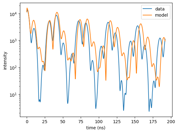
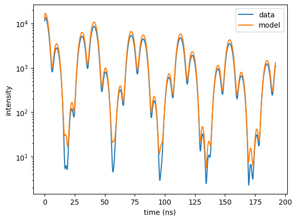
# time spectrum
sample.angle = 0.225
time_spectrum = nx.TimeSpectrum(experiment = exp,
time_length = 200,
time_step = 0.2,
bunch_spacing = 192.2, # PETRA III bunch spacing
time_data = time_data,
intensity_data = time_spec_data,
id = "time spectrum")
time_axis , intensity = time_spectrum.Calculate()
plt.semilogy(time_data, time_spec_data, label = "data")
plt.semilogy(time_axis, intensity, label = "model")
plt.legend()
plt.xlabel('time (ns)')
plt.ylabel('intensity')
plt.show()
Now, set up the multi-measurement fit. We use a local method here because the initial guess is already quite close. However, often global methods are a better option when the initial guess is far off.
fit = nx.Fit(measurements = [ref, time_spectrum])

fit.options.method = "Newuoa"

fit.Evaluate()
The last part of the output shows
Total cost = 2.271e+03

cost for each FitMeasurement is:

  no. |                           id |                cost |                   %
    0 |                 reflectivity |           4.523e+01 |               1.991
    1 |                time spectrum |           2.226e+03 |              98.009
Plot the results
plt.semilogy(angles_data, reflectivity_data, label = "data")
plt.semilogy(angles_data, ref.result, label = "model")
plt.legend()
plt.xlabel('angle (deg)')
plt.ylabel('reflectivity')
plt.show()

plt.semilogy(time_data, time_spec_data, label = "data")
plt.semilogy(time_axis, time_spectrum.result, label = "model")
plt.legend()
plt.xlabel('time (ns)')
plt.ylabel('intensity')
plt.show()
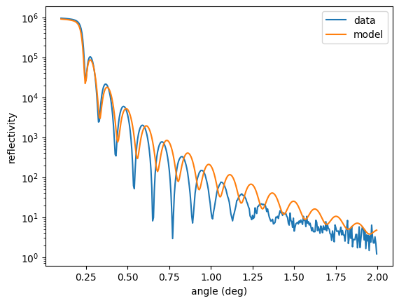
The last part of the output shows that the reflectivity only slightly contributes to the total \(cost\).
The fit of the reflectivity is not optimal due to its relatively low weight.
To improve the fit, you can change the fit_weight.
Multi-fit weighting
When fitting multiple measurements the problem arises that the intensities and number of points can be very different.
Therefore, the \(cost\) of the measurements might differ a lot and a single measurement might dominate the parameter fitting.
To tune the relative contribution of each fit you can set the fit_weight of a Measurement.
This parameter will be multiplied to the \(cost\) of the individual measurement, thus changing its weight in the total \(cost\).
Note
In principle it is possible to mix different Residual objects for different FitMeasurement objects.
Be careful when doing so because it can strongly influence the calculated \(cost\) and thus the weight in fitting.
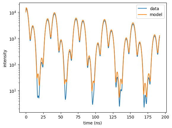
For the previous example we can change the fit weight of the reflectivity to improve the fit of the reflectivity
fit.SetInitialVars()

ref.fit_weight = 1e3

fit.Evaluate()

plt.semilogy(angles_data, reflectivity_data, label = "data")
plt.semilogy(angles_data, ref.result, label = "model")
plt.legend()
plt.xlabel('angle (deg)')
plt.ylabel('reflectivity')
plt.show()

plt.semilogy(time_data, time_spec_data, label = "data")
plt.semilogy(time_axis, time_spectrum.result, label = "model")
plt.legend()
plt.xlabel('time (ns)')
plt.ylabel('intensity')
plt.show()
to get
Total cost = 1.050e+04

cost for each FitMeasurement is:

  no. |                           id |                cost |                   %
    0 |                 reflectivity |           2.068e+03 |              19.705
    1 |                time spectrum |           8.428e+03 |              80.295
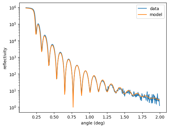
Now, the reflectivity is fit well. Its \(cost\) increased because the weighting was increased by a factor of 1000.
An even better fit is expected with a global algorithm.
Multi-fit from multiple Experiments
A typical example is to fit several Moessbauer spectra or time spectra together when an experimental parameter has been changed. Let’s assume we have changed the temperature of an experiment which will in turn affect the magnetic hyperfine field and the Lamb-Moessbauer factor. The quadrupole splitting and isomer shift should not change. This is a pure academic example, the data to be fit are generated with those assumptions. We have three different Moessbauer spectra
which we want to fit together.
In the Nexus language those are three different experiments where the external parameter (temperature) and the internal parameters (hyperfine field, Lamb Moessbauer factor) have been changed. So, we need to set up three experiments in which the hyperfine field and the Lamb-Moessbauer factor can be fit separately for each temperature.
For now we just take a simple iron sample in this example, with non realistic parameters. The hyperfine parameters are assumed to be isotropically distributed. The experiments are defined separately here, but one could also use a function to do so, see Multilayers and Nexus references.
import nexus as nx
import numpy as np
import matplotlib.pyplot as plt

# load data
data_A = np.loadtxt('spectrum_A.txt')

velocities_A = data_A[:,0]
intensity_A = data_A[:,1]

data_B = np.loadtxt('spectrum_B.txt')

velocities_B = data_B[:,0]
intensity_B = data_B[:,1]

data_C = np.loadtxt('spectrum_C.txt')

velocities_C = data_C[:,0]
intensity_C = data_C[:,1]

# setup common objects
beam = nx.Beam()
beam.Unpolarized()

# define a measurement for each temperature

# there are common fit parameters as the isomer shift and the quadrupole splitting
# they should be the same for every measurement
# so we define them independently of the measurement

isomer_for_all = nx.Var(1.1, min = 0, max = 1.2, fit = True, id = "isomer")

quadrupole_for_all = nx.Var(1.0, min = 0.5, max = 1.2, fit = True, id = "quadrupole")


# the magnetic field and the Lamb-Moessbauer factor are sample specific and have to be defined for each measurement

# ---- iron experiment at temperature A ----

site_A = nx.Hyperfine(weight = 1,
                      isomer = isomer_for_all,
                      magnetic_field = nx.Var(27, min = 15, max = 40, fit = True, id = "magnetic field A"),
                      quadrupole = quadrupole_for_all,
                      isotropic = True)

mat_iron_A = nx.Material(composition = [["Fe", 1]],
                         density = 7.8,
                         isotope = nx.lib.moessbauer.Fe57,
                         abundance = 0.02119,
                         lamb_moessbauer = nx.Var(0.81, min = 0.5, max = 1, fit = True, id = "Lamb Moessbauer A"),
                         hyperfine_sites = [site_A])

layer_iron_A = nx.Layer(thickness = 1000,
                        material = mat_iron_A)

sample_A = nx.Sample(layers = [layer_iron_A],
                     geometry = "f")

experiment_A = nx.Experiment(beam = beam,
                             objects = [sample_A],
                             isotope = nx.lib.moessbauer.Fe57)

moessbauer_spec_A = nx.MoessbauerSpectrum(experiment = experiment_A,
                                          velocity = velocities_A,
                                          intensity_data = intensity_A)


# ---- iron experiment at temperature B ----

site_B = nx.Hyperfine(weight = 1,
                      isomer = isomer_for_all,
                      magnetic_field = nx.Var(23, min = 15, max = 40, fit = True, id = "magnetic field B"),
                      quadrupole = quadrupole_for_all,
                      isotropic = True)

mat_iron_B = nx.Material(composition = [["Fe", 1]],
                         density = 7.8,
                         isotope = nx.lib.moessbauer.Fe57,
                         abundance = 0.02119,
                         lamb_moessbauer = nx.Var(0.63, min = 0.5, max = 1, fit = True, id = "Lamb Moessbauer B"),
                         hyperfine_sites = [site_B])

layer_iron_B = nx.Layer(thickness = 1000,
                        material = mat_iron_B)

sample_B = nx.Sample(layers = [layer_iron_B],
                     geometry = "f")

experiment_B = nx.Experiment(beam = beam,
                             objects = [sample_B],
                             isotope = nx.lib.moessbauer.Fe57)

moessbauer_spec_B = nx.MoessbauerSpectrum(experiment = experiment_B,
                                          velocity = velocities_B,
                                          intensity_data = intensity_B)

# ---- iron experiment at temperature C ----

site_C = nx.Hyperfine(weight = 1,
                      isomer = isomer_for_all,
                      magnetic_field = nx.Var(8, min = 0, max = 25, fit = True, id = "magnetic field C"),
                      quadrupole = quadrupole_for_all,
                      isotropic = True)

mat_iron_C = nx.Material(composition = [["Fe", 1]],
                         density = 7.8,
                         isotope = nx.lib.moessbauer.Fe57,
                         abundance = 0.02119,
                         lamb_moessbauer = nx.Var(0.6, min = 0.5, max = 1, fit = True, id = "Lamb Moessbauer C"),
                         hyperfine_sites = [site_C])

layer_iron_C = nx.Layer(thickness = 1000,
                        material = mat_iron_C)

sample_C = nx.Sample(layers = [layer_iron_C],
                     geometry = "f")

experiment_C = nx.Experiment(beam = beam,
                             objects = [sample_C],
                             isotope = nx.lib.moessbauer.Fe57)

moessbauer_spec_C = nx.MoessbauerSpectrum(experiment = experiment_C,
                                          velocity = velocities_C,
                                          intensity_data = intensity_C)

plt.plot(velocities_A, intensity_A)
plt.plot(velocities_A, moessbauer_spec_A())
plt.xlabel('velocity (mm/s)')
plt.ylabel('intensity')
plt.show()

plt.plot(velocities_B, intensity_B)
plt.plot(velocities_B, moessbauer_spec_B())
plt.xlabel('velocity (mm/s)')
plt.ylabel('intensity')
plt.show()

plt.plot(velocities_C, intensity_C)
plt.plot(velocities_C, moessbauer_spec_C())
plt.xlabel('velocity (mm/s)')
plt.ylabel('intensity')
plt.show()
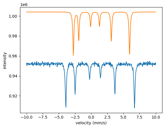
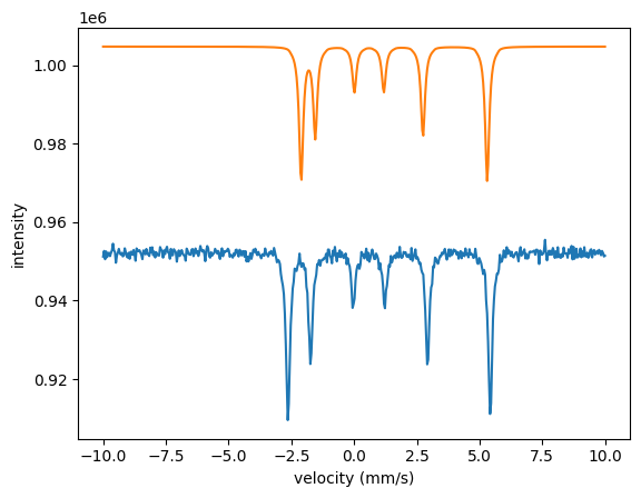
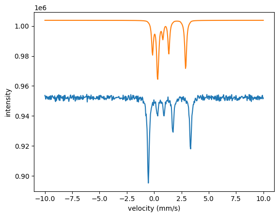
The three spectra are quite far off with the initial parameters. The local algorithms are likely to run into problems when the parameters are that far off. Let’s try the annealing algorithm.
# set up the fit
fit = nx.Fit(measurements = [moessbauer_spec_A, moessbauer_spec_B, moessbauer_spec_C])

fit.options.method = "Annealing"

fit()
The output is
Starting fit with 3 measurement data set(s) and 11 fit parameter(s).

  no. |                           id |       initial value |              min |              max
    0 |                   ES scaling |              0.9528 |                0 |            95.28
    1 |            Lamb Moessbauer A |                0.81 |              0.3 |                1
    2 |                       isomer |                   2 |                0 |                3
    3 |             magnetic field A |                  27 |                0 |               40
    4 |                   quadrupole |                 1.2 |                0 |                2
    5 |                   ES scaling |            0.952803 |                0 |          95.2803
    6 |            Lamb Moessbauer B |                0.63 |              0.3 |                1
    7 |             magnetic field B |                  23 |                0 |               40
    8 |                   ES scaling |            0.952806 |                0 |          95.2806
    9 |            Lamb Moessbauer C |                 0.4 |              0.3 |                1
   10 |             magnetic field C |                   4 |                0 |               40

Calling Pagmo solver with fit method PagmoDiffEvol

  population: 120
  iterations: 100

  cost = 1.017731e-02

Calling ceres solver with fit method LevMar

Ceres Solver Report: Iterations: 16, Initial cost: 1.017731e-02, Final cost: 1.179941e-08, Termination: CONVERGENCE

Fit performed with 11 fit parameter(s).

  no. |                           id |           fit value |       initial value |              min |              max
    0 |                   ES scaling |                   1 |              0.9528 |                0 |            95.28
    1 |            Lamb Moessbauer A |            0.795999 |                0.81 |              0.3 |                1
    2 |                       isomer |            0.999995 |                   2 |                0 |                3
    3 |             magnetic field A |                  33 |                  27 |                0 |               40
    4 |                   quadrupole |            0.799977 |                 1.2 |                0 |                2
    5 |                   ES scaling |            0.999999 |            0.952803 |                0 |          95.2803
    6 |            Lamb Moessbauer B |            0.729697 |                0.63 |              0.3 |                1
    7 |             magnetic field B |              25.002 |                  23 |                0 |               40
    8 |                   ES scaling |                   1 |            0.952806 |                0 |          95.2806
    9 |            Lamb Moessbauer C |            0.600003 |                 0.4 |              0.3 |                1
   10 |             magnetic field C |                  12 |                   4 |                0 |               40

  total cost = 1.179941e-08

cost for each FitMeasurement is:

  no. |                           id |                cost |                   %
    0 |                              |        3.439962e-11 |               0.292
    1 |                              |           1.175e-08 |              99.579
    2 |                              |           1.527e-11 |               0.129
In the last section the fit module prints the cost of the individual measurements. And plot the result
plt.plot(velocities_A, intensity_A)
plt.plot(velocities_A, moessbauer_spec_A.result)
plt.xlabel('velocity (mm/s)')
plt.ylabel('intensity')
plt.show()

plt.plot(velocities_B, intensity_B)
plt.plot(velocities_B, moessbauer_spec_B.result)
plt.xlabel('velocity (mm/s)')
plt.ylabel('intensity')
plt.show()

plt.plot(velocities_C, intensity_C)
plt.plot(velocities_C, moessbauer_spec_C.result)
plt.xlabel('velocity (mm/s)')
plt.ylabel('intensity')
plt.show()
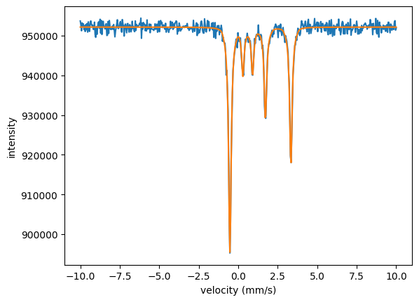
The fit nicely fitted all three spectra together. Note that the isomer shift and the quadrupole splitting are only fit once. They are the same in all three experiments.
Using scipy for fitting
Nexus covers all typical fitting scenarios to evaluate experimental data from Moessbauer science. In case you want to fit a property that is not covered you can always use scipy and its fitting algorithms. However, you are limited to the methods provided there.
Here is a basic example how to use scipy with Nexus. First, you set up your experiment and the measurements as in any other simulation.
import nexus as nx
import numpy as np
import matplotlib.pyplot as plt

from scipy.optimize import minimize
from scipy.optimize import leastsq

material_Fe = nx.Material.Template(nx.lib.material.Fe_enriched)

lay_Fe = nx.Layer(id = "Fe layer",
                  material = nx.Material.Template(nx.lib.material.Fe_enriched),
                  thickness = 10,
                  roughness = 0.1)

lay_Pt = nx.Layer(id = "Pt layer",
                  material = nx.Material.Template(nx.lib.material.Pt),
                  thickness = 15,
                  roughness = 0.1)

sub_Si = nx.Layer(id = "Si substrate",
                  material = nx.Material.Template(nx.lib.material.Si),
                  thickness = nx.inf,
                  roughness = 0.1)

sample = nx.Sample(id = "simple layers",
                   layers = [lay_Fe, lay_Pt, sub_Si],
                    geometry = "r",
                    length = 10,
                    roughness = "a")

beam  = nx.Beam(fwhm = 0.2)

exp = nx.Experiment(beam = beam,
                    objects = sample,
                    id = "my exp")

angles = np.arange(0.001, 3, 0.001)

reflectivity = nx.Reflectivity(experiment = exp,
                               sample = sample,
                               energy = nx.lib.energy.CuKalpha,  # Cu K alpha line
                               angles = angles,
                               resolution = 0.001)

reference_ref = reflectivity()

# start values for initial guess
lay_Fe.thickness = 7.3
lay_Pt.thickness = 18.9

# initial guess vector
p0 = [lay_Fe.thickness.value, lay_Pt.thickness.value]

ref = reflectivity()

plt.semilogy(angles, reference_ref)
plt.semilogy(angles, ref)
plt.xlabel('angle (deg)')
plt.ylabel('reflectivity')
plt.show()
Then, you define a target function that is to be minimized and the optimization problem.
Here’s an example for the least_squares module of scipy.
# definition of the optimization problem
def errorfunc(params, target):
    # redefine the Var values
    lay_Fe.thickness = params[0]
    lay_Pt.thickness = params[1]
    # here the reflectivity is called with the new parameters
    return reflectivity() - target

res = least_squares(errorfunc,
                    p0,
                    args=([reference_ref]),
                    method = `trf`,
                    ftol=1e-15,
                    xtol=1e-15)

print(res.x)

plt.semilogy(angles, reference_ref)
plt.semilogy(angles, reflectivity())
plt.xlabel('angle (deg)')
plt.ylabel('reflectivity')
plt.show()
and one with the minimze module of scipy
# start values for initial guess again
lay_Fe.thickness = 7.3
lay_Pt.thickness = 18.9

# initial guess vector
p0 = [lay_Fe.thickness.value, lay_Pt.thickness.value]

def errorfunc(params,target):
    # redefine the Var values
    lay_Fe.thickness = params[0]
    lay_Pt.thickness = params[1]
    # here the reflectivity is called with the new parameters
    # calculate the total cost (np.sum) for the minimize module
    return np.sum(np.square(reflectivity() - target))

res = minimize(errorfunc,
               p0,
               args = (reference_ref),
               method = 'Nelder-Mead',
               tol = 1e-6)

print(res.x)

plt.semilogy(angles, reference_ref)
plt.semilogy(angles, reflectivity())
plt.xlabel('angle (deg)')
plt.ylabel('reflectivity')
plt.show()

Note that Nexus’ referencing of the variables in different objects will still work with scipy.
Parameter constraints
New in version 1.1.0.
Nexus offers the feature to apply constraints on fit parameters. The fit function
is then subject to an arbitrary number of constraints \(g_i(x,y)\) functions. These constraints can either be of equality type \(g_i(x,y) = 0\) or of inequality type \(g_i(x,y) \geq 0\). Equality and inequality constraints can be combined
in order to specify the optimization problem. You should take care that all constraints are satisfiable simultaneously, which Nexus cannot check for you.
Equality constraints
An equality constraint
is applied via a function that is passed to the equality attribute of a Var.
The fit attribute of the Var object must be False in order to apply an equality constraint.
In order to apply a constraint you have to create a function that specifies the constraint function and apply it to the Var object.
The constraint function is given to the equality class attribute.
The functional dependence can be any (non-)linear function and can depend on several fit parameters.
Further, the constraint must be applied during the Var initialization and it must return a float value.
import nexus as nx

a = nx.Var(1, min=0, max=1, fit=True, id="a")

# the sum of a and b is restricted to 1
# The constraint g() = 0 is
# a + b - 1 = 0
# The constraint is applied to b
# b = 1 - a

# via function definition
def sum_constraint():
    return 1 - a.value

b = nx.Var(1, min=0, max=1, fit=False, equality=sum_constraint, id="b")

# or via lambda function
b = nx.Var(1, min=0, max=1, fit=False, equality=lambda: 1 - a.value, id="b")
These constraints can be used to couple fit parameters.
They also offer the possibility to use external fit parameters.
Those are Var objects that are not assigned to other Nexus objects.
It offers the possibility to fit theoretical models directly to the measured data sets.
Equality constraints on Vars
This example shows the basic usage of equality constraints.
Here, two hyperfine sites will be fit to this spectrum and the magnetic fields of the two sites are coupled.
import nexus as nx
import numpy as np

# load the example spectrum
detuning, intensity = nx.data.Load("spectrum_equality.txt",
                                    x_index = 0,
                                    intensity_index = 1)

# setup fit parameters with initial guess
# and create dependent Vars
isomer = nx.Var(0.8, min = 0, max = 2, fit = True, id="isomer")

mag_1 = nx.Var(value = 32, min = 25, max = 35, fit = True, id = "mag field 1")

# we assume that the magnetic fields of the two sites have a difference of 23 T
# mag2 = mag1 - 23
def equality_mag2():
    return mag_1.value - 23

# we apply a value of 14 that is used for all regular calculations.
# for fitting, the equality constraint function equality_mag2 is applied and the value is ignored.
mag_2 = nx.Var(value = 14, equality = equality_mag2, id = "mag field 2")

# assign to sites
site1 = nx.Hyperfine(
    id = "site 1",
    weight = 0.5,
    isomer = isomer,
    magnetic_field = mag_1,
    isotropic = False)

site2 = nx.Hyperfine(
    id = "site 2",
    weight = 0.5,
    isomer = isomer,
    magnetic_field = mag_2,
    isotropic = False)


#setup experiment
lay_Fe = nx.Layer(id = "Fe",
                  material = nx.Material.Template(nx.lib.material.Fe_enriched),
                  thickness = 3000)

lay_Fe.material.hyperfine_sites = [site1, site2]

sample = nx.Sample(id = "sample",
                   layers = [lay_Fe],
                   geometry = "f")

beam  = nx.Beam()
beam.LinearSigma()

exp = nx.Experiment(beam = beam,
                    objects = [sample],
                    isotope = nx.moessbauer.Fe57,
                    id = "my exp")

energy_spec = nx.EnergySpectrum(exp,
                                detuning,
                                intensity_data = intensity,
                                id = "energy spec")

energy_spec()
energy_spec.Plot()
and obtain the initial guess of your fit.
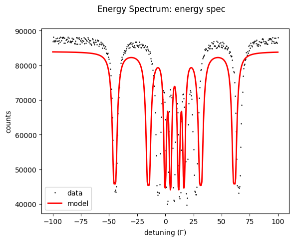
Note that for calculations (not fitting) always the provided value for the dependent variable is used. Equality constraints are only used for fitting.
fit = nx.Fit([energy_spec], id = "fit")
fit()

energy_spec.Plot()
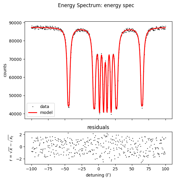
Note that you obtain the following lines
Fit performed with 4 fit parameter(s).

  no. |                           id |           fit value |       initial value |              min |              max
    0 |                   ES scaling |             99814.5 |             88182.9 |                0 |      8.81829e+06
    1 |                    ES backgr |             1151.94 |             7777.25 |                0 |           777725
    2 |                       isomer |             1.00012 |                 0.8 |                0 |                2
    3 |                  mag field 1 |             33.0028 |                  32 |               25 |               35

and 1 equality constraint(s) on parameter(s).

  no. |                           id |               value
    0 |                  mag field 2 |             10.0028
where you can observe that the mag field 2 is fit with the provided difference of 23 T to mag field 1.
Equality constraint with parameters
Equality constraint functions normally have simple mathematical relations between Var objects, like
a = nx.Var(5, min = 0, max = 10, fit = True, id = "a")
b = nx.Var(3, min = 0, max = 10, fit = True, id = "b")

def equality_constraint():
    return a.value + 2 * b.value

c = nx.Var(0, equality = equality_constraint, id = "c")
However, equality constraints can also depend on variables like any other function.
a = nx.Var(5, min = 0, max = 10, fit = True, id = "a")
b = nx.Var(3, min = 0, max = 10, fit = True, id = "b")

def equality_constraint(scaling):
    return a.value + scaling * b.value
Now, the problem is that the parameter cannot easily passed to the dependent Var c.
The equality attribute only takes functions as input.
Writing equality = equality_constraint(2) is not valid as it returns a float and not a function.
The correct way is to use a Python lambda function.
It will create a function reference which calls your equality constraint function with the passed arguments.
c = nx.Var(0, equality = lambda: equality_constraint(2), id = "c")

# or

x = 2
c = nx.Var(0, equality = lambda: equality_constraint(x), id = "c")
Equality functions can have as many parameters as needed.
Inequality constraints
Inequality constraints
are applied to the Fit or Optimizer module via the inequalites attribute.
The user has to define inequality constraints as functions and pass them as a list.
For example, two inequality constraints are implemented like this
import nexus as nx

a = nx.Var(1, min=0, max=1, fit=True, id="a")
b = nx.Var(1, min=0, max=1, fit=True, id="b")
c = nx.Var(2, min=0, max=4, fit=True, id="c")

#define two inequality constraints

# via function definition
def ineq1():
    return a.value > b.value

def ineq2():
    return b.value**2 + c.value**2 > 1

fit = nx.Fit(measurements= [measurements],
             inequalities = [ineq1, ineq2])

# or via lambda functions
fit = nx.Fit(measurements= [measurements],
             inequalities = [lambda: a.vlaue > b.value,
                             lambda: b.value**2 + c.value**2 > 1])
As an example we will use the same fit with two hyperfine sites as in the first examples of the equality constraints. This time we want to ensure that the magnetic field of site 2 is larger than the one of site 1. For local algorithms you have to ensure that the starting conditions is satisfied otherwise the fit will not run. For global algorithms it is not necessary. However, the ranges must be large enough for the inequality constraints to be satisfiable.
import nexus as nx

# load example spectrum
detuning, intensity = nx.data.Load("spectrum_equality.txt",
                                   x_index = 0,
                                   intensity_index = 1)

#setup experiment
isomer = nx.Var(0.8, min = 0, max = 2, fit = True, id="isomer")

site1 = nx.Hyperfine(
    id = "site 1",
    weight = 0.5,
    isomer = isomer,
    magnetic_field = nx.Var(value = 32, min = 0, max = 35, fit = True, id = "mag field 1"),
    isotropic = False)

site2 = nx.Hyperfine(
    id = "site 2",
    weight = 0.5,
    isomer = isomer,
    magnetic_field = nx.Var(value = 14, min = 0, max = 35, fit = True, id = "mag field 2"),
    isotropic = False)

mat_Fe = nx.Material.Template(nx.lib.material.Fe_enriched)

mat_Fe.hyperfine_sites = [site1, site2]

#create sample
lay_Fe = nx.Layer(id = "Fe",
                  material = mat_Fe,
                  thickness = 2800)

sample = nx.Sample(id = "sample",
                   layers = [lay_Fe],
                   geometry = "f")

beam  = nx.Beam()

exp = nx.Experiment(beam = beam,
                    objects = [sample],
                    isotope = nx.moessbauer.Fe57,
                    id = "my exp")

energy_spec = nx.EnergySpectrum(exp,
                                detuning,
                                intensity_data = intensity,
                                id = "energy spec")
# fit with inequality
fit = nx.Fit([energy_spec],
             # magnetic field of site1 must be smaller than that of site 2
             inequalities = [lambda: site1.magnetic_field.value < site2.magnetic_field.value])

fit.options.method = "PagmoDiffEvol"

fit()
The fit takes the inequality constraint into account and print
Fit performed with 5 fit parameter(s):

  no. |                           id |           fit value |       initial value |              min |              max
    0 |                   ES scaling |             99939.1 |             88182.9 |                0 |      8.81829e+06
    1 |                    ES backgr |                   0 |             7777.25 |                0 |           777725
    2 |                       isomer |             1.00017 |                 0.8 |                0 |                2
    3 |                  mag field 1 |             9.99519 |                  32 |                0 |               35
    4 |                  mag field 2 |             33.0031 |                  14 |                0 |               35

and 0 equality constraint(s) on parameter(s):

and 1 inequality constraint(s).
Magnetic field of site 1 is indeed smaller than that of site 2.
External fit variables
The equality attribute can also be used to couple Var objects to one or various external fit parameters.
External fit parameter are all Var objects that are not assigned to other Nexus object directly, like Hyperfine, Layer, Distribution, Sample and so on, and are used in an equality constraint of a Var.
This external dependence is helpful in case a functional dependence on an external parameter or model should be fit to data.
To do so, one has to create a Var object that is your free parameter and create a couple of dependent Var objects.
The free parameter has to be registered via the external_fit_variables attribute of the Fit or Optimizer.
A simple example is the fit of two sites as shown before.
This time we do not put a constraint on the variable in depedence on another assigned Var (mag_field_1 in the previous example) but use of an external fit variable on the magnetic field of the second site.
import nexus as nx
import numpy as np

# load example specturm
detuning, intensity = nx.data.Load("spectrum_equality.txt",
                                    x_index = 0,
                                    intensity_index = 1)


#setup fit parameters
isomer = nx.Var(0.8, min = 0, max = 2, fit = True, id="isomer")

mag_1 = nx.Var(value = 32, min = 25, max = 35, fit = True, id = "mag field 1")

# create a Var used as external fit parameter
# it is not assigned to a Nexus object directly
external_fit_mag_2 = nx.Var(value = 12, min = 8, max = 15, fit = True, id = "ext mag field 2")

# a simple functional dependence on the external fit parameter
def external_func_mag2():
    return external_fit_mag_2.value

# assign to sites
site1 = nx.Hyperfine(
    id = "site 1",
    weight = 0.5,
    isomer = isomer,
    magnetic_field = mag_1,
    isotropic = False)

site2 = nx.Hyperfine(
    id = "site 2",
    weight = 0.5,
    isomer = isomer,
    magnetic_field = nx.Var(value = 14, equality = external_func_mag2, id = "mag field 2"),
    isotropic = False)

#create sample
lay_Fe = nx.Layer(id = "Fe",
                  material = nx.Material.Template(nx.lib.material.Fe_enriched),
                  thickness = 3000)

lay_Fe.material.hyperfine_sites = [site1, site2]

sample = nx.Sample(id = "sample",
                   layers = [lay_Fe],
                   geometry = "f")

beam  = nx.Beam()
beam.LinearSigma()

exp = nx.Experiment(beam = beam,
                    objects = [sample],
                    isotope = nx.moessbauer.Fe57,
                    id = "my exp")

energy_spec = nx.EnergySpectrum(exp,
                                detuning = detuning,
                                intensity_data = intensity,
                                id = "energy spec")

energy_spec()
energy_spec.Plot()

# assign the external_fit_parameter to the Fit object.
fit = nx.Fit([energy_spec],
             external_fit_variables = [external_fit_mag_2])

fit()

energy_spec.Plot()
The plot of the fit is the same as before. The important output of the fit is
Fit performed with 5 fit parameter(s).

  no. |                           id |           fit value |       initial value |              min |              max
    0 |                   ES scaling |             99815.5 |             88182.9 |                0 |      8.81829e+06
    1 |                    ES backgr |             1151.14 |             7777.25 |                0 |           777725
    2 |                       isomer |             1.00013 |                 0.8 |                0 |                2
    3 |                  mag field 1 |             33.0017 |                  32 |               25 |               35
    4 |              ext mag field 2 |             10.0033 |                  12 |                8 |               15

and 1 equality constraint(s) on parameter(s).

  no. |                           id |               value
    0 |                  mag field 2 |             10.0033
You can see that the mag field 2 is recognized as an equality constraint and the ext mag field 2 is a fit variable.
Both have exactly the same value as expected.
Importantly the external fit parameter is the one that is fit.
This simple example is trivial but it shows how external fit parameters are used.
Fit to external models
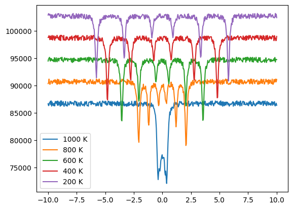
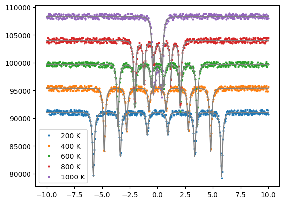
Equality constraints and external fit parameters can be used to fit data sets to models on any parameters, most typically hyperfine parameters. Here, we show how various external parameters can be used to fit data sets directly to an external model. For example, you have several measurements at different temperatures of an iron film and you want to directly fit a Bloch T 3/2 law to the data. This is just an example for demonstration purposes.
In the Nexus language it is a multi-measurement fit from several experiments.
We have to setup an experiment for each measurement and connect it to a Bloch law function whose parameters should be fit.
The spectra used for the different temperatures are 1000 K, 800 K, 600 K, 400 K, 200 K
First, we load all data
import nexus as nx
import numpy as np
import matplotlib.pyplot as plt

vel_1000, int_1000 = nx.data.Load("spectrum_1000K.txt", x_index = 0, intensity_index = 1)
vel_800, int_800 = nx.data.Load("spectrum_800K.txt", x_index = 0, intensity_index = 1)
vel_600, int_600 = nx.data.Load("spectrum_600K.txt", x_index = 0, intensity_index = 1)
vel_400, int_400 = nx.data.Load("spectrum_400K.txt", x_index = 0, intensity_index = 1)
vel_200, int_200 = nx.data.Load("spectrum_200K.txt", x_index = 0, intensity_index = 1)

plt.plot(vel_1000, int_1000, label = "1000 K")
plt.plot(vel_800, int_800 + 4e3, label = "800 K")
plt.plot(vel_600, int_600 + 8e3, label = "600 K")
plt.plot(vel_400, int_400 + 12e3, label = "400 K")
plt.plot(vel_200, int_200 + 16e3, label = "200 K")
plt.legend()
plt.show()
Then, we set up the external model we want to fit.
# Bloch T^3/2 function
# M(T) = M(0)* (1-(T/Tc)^3/2)

# create external fit parameters
Tc = nx.Var(1040, min = 1000, max= 1100, fit = True, id = "Tc")
M_0 = nx.Var(40, min = 30, max= 50, fit = True, id ="mag_0")
exponent = nx.Var(1.2, min = 1, max= 2, fit = True,id = "exp")

# Only the temperature T is known from the experiment and will be set.
def Bloch(T):
    # return a magnetic field value in Tesla
    return M_0.value * (1 - (T/Tc.value)**(exponent.value))
To create such an amount of measurement spectra we use a function to create them.
# create the experiment in a for loop
# we assume that the oterh hyperfine parameters do not change individually
# we also want to fit the isomer shift as a common variable to all measurements
isomer_shift = nx.Var(0.5, min = -1, max = 1, fit = True, id = "isomer all")

# It is also possible to create additional Vars
# either in the function to be fit individually

# we can use the same beam object in each experient
beam = nx.Beam()
beam.Unpolarized()

# because the hyperfine parameters change we have to create
# new samples, experiments and MoessbauerSpectra for each temperature
# also we have to pass the experimental temperature and velocity and intensity data
def setup_specturm(temperature, velocity_data, intensity_data):
    site = nx.Hyperfine(weight=1,
      isomer = isomer_shift,
      # now assign the external function to the magnetic field of each experiment
      # given by the Bloch function and the set temperature
      magnetic_field = nx.Var(0, id="mag_at_"+str(temperature), equality = lambda: Bloch(temperature)),
      isotropic = True)

    mat_Fe = nx.Material.Template(nx.lib.material.Fe)

    mat_Fe.hyperfine_sites = [site]

    layer_Fe = nx.Layer(id = "Fe",
                        material = mat_Fe,
                        thickness = 3000)

    sample = nx.Sample(layers = [layer_Fe])

    exp = nx.Experiment(beam = beam,
                        objects = [sample],
                        isotope = nx.lib.moessbauer.Fe57)

    spectrum = nx.MoessbauerSpectrum(experiment = exp,
                                     velocity = velocity_data,
                                     intensity_data = intensity_data)

    return spectrum
and create all needed measurements
# create list to loop over
temps = [200, 400, 600, 800, 1000]
vels = [vel_200, vel_400, vel_600, vel_800, vel_1000]
dats = [int_200, int_400, int_600, int_800, int_1000]
measurements = []

# create all spectra and append to list
for t, v, d in zip(temps, vels, dats):
    measurements.append(setup_specturm(t,v,d))
At last we set up the fit model with the external fit variables
fit = nx.Fit(measurements = measurements,
             id = "Bloch fit",
             external_fit_variables = [Tc, M_0, exponent])

fit()
to obtain the fit results. Part of the output is
Fit performed with 14 fit parameter(s).

  no. |                           id |           fit value |       initial value |              min |              max
    0 |                   ES scaling |              100190 |               87188 |                0 |       8.7188e+06
    1 |                    ES backgr |             333.481 |             8601.76 |                0 |           860176
    2 |                   isomer all |        -5.12588e-05 |                 0.5 |               -1 |                1
    3 |                   ES scaling |              100621 |               87193 |                0 |       8.7193e+06
    4 |                    ES backgr |                   0 |             8603.46 |                0 |           860346
    5 |                   ES scaling |               99477 |               87191 |                0 |       8.7191e+06
    6 |                    ES backgr |             956.819 |             8603.12 |                0 |           860312
    7 |                   ES scaling |              100333 |               87188 |                0 |       8.7188e+06
    8 |                    ES backgr |             200.076 |             8600.74 |                0 |           860074
    9 |                   ES scaling |              100459 |               87195 |                0 |       8.7195e+06
   10 |                    ES backgr |             111.197 |             8604.11 |                0 |           860411
   11 |                           Tc |             1043.07 |                1040 |             1000 |             1100
   12 |                          M_0 |              39.126 |                  40 |               30 |               50
   13 |                     exponent |             1.49986 |                 1.2 |                1 |                2

and 5 equality constraint(s) on parameter(s).

  no. |                           id |               value
    0 |                   mag_at_200 |             35.8402
    1 |                   mag_at_400 |             29.8333
    2 |                   mag_at_600 |             22.0552
    3 |                   mag_at_800 |             12.8448
    4 |                  mag_at_1000 |              2.3981
The magnetic fields at different temperatures are calculated from the Bloch function and are dependent parameters via the equality constraints.
The external fit parameters of the Bloch functions Tc, M_0, exponent are fit.
To plot the data use
offset = 0
for t, v, d, m in zip(temps, vels, dats, measurements):
    int = m.Calculate()
    offset += max(int) * 0.05
    plt.plot(v, d + offset, label = str(t)+" K", marker='o', markersize = 2, linewidth=0)
    plt.plot(v, int + offset, color='grey')

plt.legend()
plt.show()
Optimizer
The Optimizer module can be used to design the experimental parameters to certain target values.
The options controlling the optimization process are the same as for the Fit module and are controlled by the OptimizerOptions class, see OptimizerOptions.
In order to perform an optimization you must define your optimizer class that is derived from the Nexus Optimizer class and holds the actual implementation of the residual to be minimized or maximized.
First, the experiment and the method are defined as in any simulation or fit.
All parameters to be optimized have to be defined as Var objects with their fit set to True.
Note
When using an Optimizer the scaling of a measurement is not fit.
Note
The optimizer always squares the residual provided by the user. So, all algorithms in Nexus solve a least square problem.
Warning
In case the optimizer is not working and python crashes it’s most likely that you have an error in your implementation of the Residual() function.
As this function is called from the C++ implementation you do not get the typical Python error message.
Look out for parts of your code that can give unexpected output and use print() in the Residual function to see if your implementation works.
A simple example
Let’s implement the trivial example mentioned at the beginning. The resonant intensity transmitted through an iron foil should be minimized.
import nexus as nx
import numpy as np
import matplotlib.pyplot as plt

# ------------------------- Fe layer --------------------------
# the thickness is initialized to be fitted
# set with boundaries between 0 and 10.000
lay_Fe = nx.Layer(id = "Fe",
                  material = nx.Material.Template(nx.lib.material.Fe_enriched),
                  thickness = nx.Var(2000, 0, 1e5, True))

site = nx.Hyperfine(magnetic_field = 33)

lay_Fe.material.hyperfine_sites = [site]

sample = nx.Sample(id = "simple layer",
                   layers = [lay_Fe],
                   geometry = "f")

beam  = nx.Beam()
beam.LinearSigma()

exp = nx.Experiment(beam = beam,
                    objects = sample,
                    isotope = nx.lib.moessbauer.Fe57,
                    id = "my exp")

detuning = np.arange(-200, 200.1, 0.2)

energy_spec = nx.EnergySpectrum(exp,
                                detuning,
                                electronic = True)

intensity = energy_spec()

plt.plot(detuning, intensity)
plt.xlabel('detuning (Gamma)')
plt.ylabel('rel. transmission')
plt.show()

print(min(intensity))
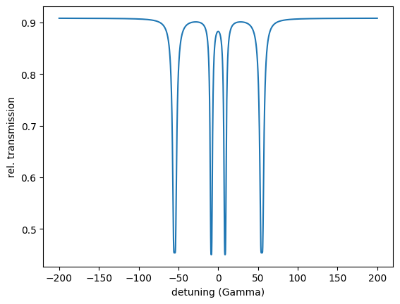
The print shows 0.45013002160328575 the minimum of the resonant intensity.
We want to optimize the thickness within the given boundaries such that this value is minimized.
We already know what will happen.
The thickness will increase because the intensity then further drops.
But let the optimizer do the job for us.
We need a class implementation with the implementation of the residual to be minimized.
# define your own Optimizer derived from nx.Optimizer
class NexusOptimizer(nx.Optimizer):
    # this is just the standard initialization of the class
    # keep it like this
    def __init__(self, measurements, id):
        super().__init__(measurements, id)

    # the implementation of the residual, the value to be minimized
    def Residual(self):
        # here we need to calculate the energy spectrum and get its minimum
        intensity = energy_spec()
        # the residual is 'min(intensity) - 0' because we target the intensity minimum to be zero (minimized)
        residual = min(intensity)
        return residual

# initialize the optimizer with the method(s) to be used in the optimizer implementation
optimizer = NexusOptimizer(measurements = [energy_spec],
                           id = "opt id")

# let's see what the residual returns
print(optimizer.Residual())  # 0.45013002160328575

# run the optimization
optimizer.Evaluate()  # or simply call optimizer()
You get similar output as for the Fit module.
User residual start value: 0.450130
Starting optimizer with 1 provided measurement dependencies and 1 fit parameter(s).
no. | id | initial value | min | max
0 | | 2000 | 0 | 100000
Calling ceres solver with optimizer method LevMar
Ceres Solver Report: Iterations: 16, Initial cost: 1.013085e-01, Final cost: 1.860658e-06, Termination: CONVERGENCE
Optimizer finished with 1 fit parameter(s).
no. | id | fit value | initial value | min | max
0 | | 100000 | 2000 | 0 | 100000
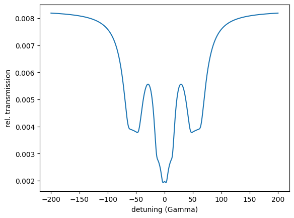
Optimized user residual from 0.45013 to 0.00192907
As expected the thickness of the film is optimized to the maximum boundary of 10000.
The optimizer also outputs the optimized residual value 0.00192907.
Let’s plot the ‘optimized’ spectrum.
plt.plot(detuning, energy_spec.result)
plt.xlabel('detuning (Gamma)')
plt.ylabel('rel. transmission')
plt.show()
Optimizing for critical coupling of a cavity
In this example we will cover a typical problem encountered in cavity structures. The topmost layer must be optimized in its thickness to ensure critical coupling into the cavity. Here, we will optimize critical coupling to the first waveguide mode.
We setup the cavity without knowing the correct thickness of the top layer.
import nexus as nx
import numpy as np
import matplotlib.pyplot as plt
from scipy.signal import find_peaks

# ------------------------- layers --------------------------

# the initial guess for the top layer is 3 nm here
# set it to a Var object with reasonable bounds
lay_Pt_top = nx.Layer(id = "Pt top",
                      material = nx.Material.Template(nx.lib.material.Pt),
                      thickness = nx.Var(3, min = 0, max = 10, fit = True, id = "Pt top thickness"))

lay_B4C = nx.Layer(id = "B4C",
                   material = nx.Material.Template(nx.lib.material.B4C),
                   thickness = 15)

lay_Fe = nx.Layer(id = "Fe",
                  material = nx.Material.Template(nx.lib.material.Fe_enriched),
                  thickness = 2)

lay_Pt_bottom = nx.Layer(id = "Pt bottom",
                         material = nx.Material.Template(nx.lib.material.Pt),
                         thickness = 15)

lay_substrate = nx.Layer(id = "substrate",
                         material = nx.Material.Template(nx.lib.material.Si),
                         thickness = nx.inf)

sample = nx.Sample(id = "cavity",
                   layers = [lay_Pt_top,
                             lay_B4C,
                             lay_Fe,
                             lay_B4C,
                             lay_Pt_bottom,
                             lay_substrate],
                   geometry = "r")

beam  = nx.Beam()
beam.LinearSigma()

exp = nx.Experiment(beam = beam,
                    objects = sample,
                    id = "my exp")

# initialize a reflectivity object used for the optimization
angles = np.linspace(0.01, 0.4, 1001)

reflectivity = nx.Reflectivity(experiment = exp,
                               sample = sample,
                               energy = nx.lib.energy.Fe57,
                               angles = angles)

intensity = reflectivity()

plt.semilogy(angles, intensity)
plt.xlabel('angle (deg)')
plt.ylabel('reflectivity')
plt.show()
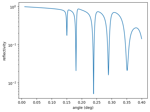
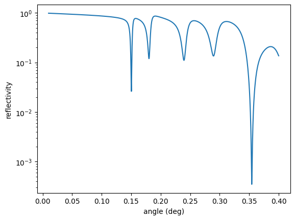
Here you see the reflectivity before optimization. The first minimum is not in the critical coupling condition as observed from the rather small decrease of the intensity. Let’s optimize.
# setup the optimizer
class NexusOptimizer(nx.Optimizer):
    def __init__(self, measurements, id):
        super().__init__(measurements, id)

    # the definition of the residual calculation
    def Residual(self):
        # calculate the reflectivity
        intensity = reflectivity()

        # get the index of the first minimum
        if (len(find_peaks(-intensity)[0]) < 1):
            return 1e30  # return large punish value
        min_index = find_peaks(-intensity)[0][0]

        # optimize for the intensity at the first minimum position
        # minimize so 'intensity - 0'
        residual = intensity[min_index]
        return residual

# pass the reflectivity object to the optimizer
opt = NexusOptimizer(measurements = [reflectivity],
                     id = "opt id")

# let's just use a local gradient-free algorithm here
opt.options.method = "Subplex"

# run the optimization
opt.Evaluate()  # or simply call opt()

plt.semilogy(angles, reflectivity.result)
plt.xlabel('angle (deg)')
plt.ylabel('reflectivity')
plt.show()
The output is
User residual start value: 0.174367

Starting optimizer with 1 provided measurement dependencies and 1 fit parameter(s).

  no. |                           id |       initial value |              min |              max
    0 |             Pt top thickness |                   3 |                0 |               10

Calling NLopt solver with optimizer method Subplex

Termination: parameter tolerance reached.
  cost = 1.310289e-02
  iterations: 50

Optimizer finished with 1 fit parameter(s).

  no. |                           id |           fit value |       initial value |              min |              max
    0 |             Pt top thickness |             2.00665 |                   3 |                0 |               10

Optimized user residual from 0.174367 to 0.0262058
The top layer thickness is optimized to 2.00665 nm.
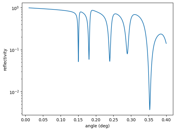
Optimizing multiple parameters in parallel
In order to optimize for several parameters in parallel we try to obtain a coupling such that the sum of the 1st and 3rd minimum of the cavity is minimal.
We take the same cavity as before
import nexus as nx
import numpy as np
import matplotlib.pyplot as plt
from scipy.signal import argrelextrema

# ------------------------- layers --------------------------

# the initial guess for the top layer is 3 nm here
# set it to a Var object with reasonable bounds
lay_Pt_top = nx.Layer(id = "Pt top",
                      material = nx.Material.Template(nx.lib.material.Pt),
                      thickness = nx.Var(3, min = 0, max = 10, fit = True, id = "Pt top thickness"))

lay_B4C = nx.Layer(id = "B4C",
                   material = nx.Material.Template(nx.lib.material.B4C),
                   thickness = 15)

lay_Fe = nx.Layer(id = "Fe",
                  material = nx.Material.Template(nx.lib.material.Fe_enriched),
                  thickness = 2)

lay_Pt_bottom = nx.Layer(id = "Pt bottom",
                         material = nx.Material.Template(nx.lib.material.Pt),
                         thickness = 15)

lay_substrate = nx.Layer(id = "substrate",
                         material = nx.Material.Template(nx.lib.material.Si),
                         thickness = nx.inf)

sample = nx.Sample(id = "cavity",
                   layers = [lay_Pt_top,
                             lay_B4C,
                             lay_Fe,
                             lay_B4C,
                             lay_Pt_bottom,
                             lay_substrate],
                   geometry = "r")

beam  = nx.Beam()
beam.LinearSigma()

exp = nx.Experiment(beam = beam,
                    objects = sample,
                    id = "my exp")

# initialize a reflectivity object used for the optimization
angles = np.linspace(0.01, 0.4, 1001)

reflectivity = nx.Reflectivity(experiment = exp,
                               sample = sample,
                               energy = nx.lib.energy.Fe57,
                               angles = angles)
Now the residual has to be changed to optimize both minima
# setup the optimizer
class NexusOptimizer(nx.Optimizer):
    def __init__(self, measurements, id):
        super().__init__(measurements, id)

    # the defienition of the residual calculation
    def Residual(self):
        # calculate the reflectivity
        intensity = reflectivity()

        # get the index of the 1st minimum
        min_index_1st = np.squeeze(argrelextrema(intensity, np.less))[0]

        # get the index of the 3rd minimum
        min_index_3rd = np.squeeze(argrelextrema(intensity, np.less))[2]

        # optimize for the intensity at both positions
        # we cannot pass several residuals to the optimizer
        # so we have to take care how to define the residual here
        # actually we have two residuals r_1 = min_1st - 0
        # and r_3  = min_3rd - 0
        # when several residuals are passed a single sum square the residuals
        # r = (min_1st - 0)^2 + (min_3rd - 0)^2
        # the squares are important if negative differences can occur
        # this passed residual is again squared by the optimizer
        # so one could pass r = \sqrt( (min_1st - 0)^2 + (min_3rd - 0)^2 )
        # but it will make no difference
        residual = intensity[min_index_1st]**2 + intensity[min_index_3rd]**2
        return residual

# pass the reflectivity object to the optimizer
opt = NexusOptimizer(measurements = [reflectivity],
                     id = "opt id")

opt.options.method = "LevMar"

# run the optimization
opt.Evaluate()  # or simply call opt()

plt.semilogy(angles, reflectivity.result)
plt.xlabel('angle (deg)')
plt.ylabel('reflectivity')
plt.show()
User residual start value: 0.030430

Starting optimizer with 1 provided measurement dependencies and 1 fit parameter(s).

  no. |                           id |       initial value |              min |              max
    0 |             Pt top thickness |                   3 |                0 |               10

Calling ceres solver with optimizer method LevMar

Ceres Solver Report: Iterations: 12, Initial cost: 4.629876e-04, Final cost: 1.473811e-05, Termination: CONVERGENCE

Optimizer finished with 1 fit parameter(s).

  no. |                           id |           fit value |       initial value |              min |              max
    0 |             Pt top thickness |             2.36109 |                   3 |                0 |               10

Optimized user residual from 0.0304298 to 0.0054292
Now, the optimized thickness is 2.36109 nm.
Note
In multi-parameter optimization square each individual residual, then take the sum as the total residual.
You might also want to add a weight to each residual. In this case the code would change to
residual = 0.4 * intensity[min_index_1st]**2 + 0.6 * intensity[min_index_3rd]**2
in case of a 40% to 60% weighting.
Optimization of a cavity spectrum
In this example a whole cavity spectrum should be optimized to a certain shape. This is a more advanced optimization problem but will serve as an example on how to optimize more than just a a few parameters.
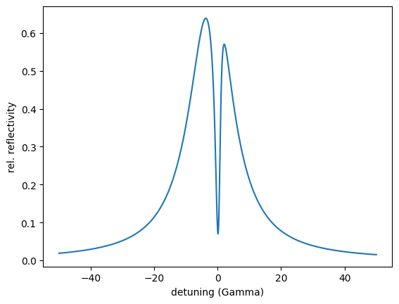
Here we want to obtain an EIT (electromagnetically induced transparency) spectrum of a cavity with a certain shape.
The spectral shape we want to create is reference_spectrum. The first column is the detuning and the second one the intensity.
import nexus as nx
import numpy as np
import matplotlib.pyplot as plt
from scipy.signal import argrelextrema

data = np.loadtxt('reference_spectrum.txt')

detuning_reference = data[:,0]
intensity_reference = data[:,1]

plt.plot(detuning_reference, intensity_reference)
plt.xlabel('detuning (Gamma)')
plt.ylabel('rel. reflectivity')
plt.show()
We set up an EIT cavity with two resonant layers. Let’s say we only have a rough guess of the thicknesses needed in the specific layers. So we set up a cavity and look at the field distribution inside the cavity and of course at the spectrum
# ------------------------- layers --------------------------
lay_Fe_top = nx.Layer(id = "Fe top",
                  material = nx.Material.Template(nx.lib.material.Fe_enriched),
                  thickness = 1)

lay_Fe_bottom = nx.Layer(id = "Fe bottom",
                  material = nx.Material.Template(nx.lib.material.Fe_enriched),
                  thickness = 1)

site = nx.Hyperfine(id = "no interactions")

lay_Fe_top.material.hyperfine_sites = [site]

lay_Fe_bottom.material.hyperfine_sites = [site]


lay_B4C_top = nx.Layer(id = "B4C top",
                   material = nx.Material.Template(nx.lib.material.B4C),
                   thickness = nx.Var(value = 4, min = 0, max = 10, fit = True, id = "B4C top"))

lay_B4C_mid = nx.Layer(id = "B4C mid",
                   material = nx.Material.Template(nx.lib.material.B4C),
                   thickness = nx.Var(value = 4, min = 0, max = 10, fit = True, id = "B4C mid"))

lay_B4C_bottom = nx.Layer(id = "B4C bottom",
                   material = nx.Material.Template(nx.lib.material.B4C),
                   thickness = nx.Var(value = 16, min = 0, max = 20, fit = True, id = "B4C top"))

lay_Pt_top = nx.Layer(id = "Pt top",
                      material = nx.Material.Template(nx.lib.material.Pt),
                      thickness = nx.Var(3.2, min = 0, max = 10, fit = True, id = "Pt top thickness"))

lay_Pt_bottom = nx.Layer(id = "Pt bottom",
                         material = nx.Material.Template(nx.lib.material.Pt),
                         thickness = 15)


lay_substrate = nx.Layer(id = "substrate",
                         material = nx.Material.Template(nx.lib.material.Si),
                         thickness = nx.inf)

cavity = nx.Sample(id = "cavity",
                   geometry = "r",
                   layers = [lay_Pt_top,
                             lay_B4C_top,
                             lay_Fe_top,
                             lay_B4C_mid,
                             lay_Fe_bottom,
                             lay_B4C_bottom,
                             lay_Pt_bottom,
                             lay_substrate],
                   angle = 0.1505)

beam  = nx.Beam()
beam.LinearSigma()

exp = nx.Experiment(beam = beam,
                    objects = cavity,
                    isotope = nx.lib.moessbauer.Fe57,
                    id = "my exp")

# initialize a reflectivity object used for the optimization
angles = np.linspace(0.01, 0.4, 1001)

reflectivity = nx.Reflectivity(experiment = exp,
                               sample = cavity,
                               energy = nx.lib.energy.Fe57,
                               angles = angles)

intensity = reflectivity()

# find third minimum
min_index = np.squeeze(argrelextrema(intensity, np.less))[2]

# set cavity angle to angle of third minimum
cavity.angle = angles[min_index]

# calcualte field intensity inside the sample
field_int = nx.FieldIntensity(sample = cavity,
                              energy = nx.moessbauer.Fe57.energy,
                              points = 1001)

depth, int = field_int()

plt.plot(depth, int)

# add lines and labels
axes = plt.gca()
y_min, y_max = axes.get_ylim()
plt.vlines(cavity.Interfaces(), y_min, y_max, colors='g', linestyles='dashed')
for id, location in zip(cavity.Ids(), np.array(cavity.Interfaces()) + 0.5):
    plt.text(location, y_max, id, fontsize = 10)
    y_max = y_max - 0.5

plt.xlabel('depth (nm)')
plt.ylabel('relative intensity')
plt.show()
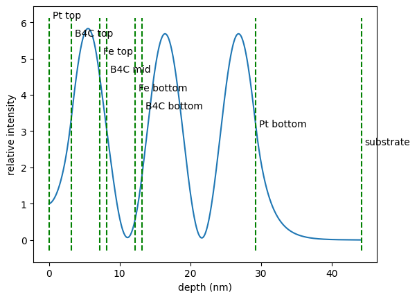
The iron layers are not at the node and antinode positions of the field inside the cavity. We do not expect a pronounced EIT effect in the spectrum. Let’s check.
energy_spectrum = nx.EnergySpectrum(experiment = exp,
                                    detuning = detuning_reference,
                                    electronic = True,
                                    id = "my energy spectrum")

intensity = energy_spectrum.Calculate()

plt.plot(detuning, intensity)
plt.xlabel('detuning (Gamma)')
plt.ylabel('rel. reflectivity')
plt.show()
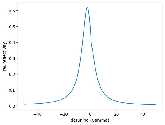
Indeed, the target spectrum looks much different. So we try to optimize.
Remember that we might need to care about certain special conditions that could crash our residual implementation.
In the following, a crash can happen if there is no third minimum in the argrelextrema function.
# setup the optimizer
class NexusOptimizer(nx.Optimizer):
    def __init__(self, measurements, id):
        super().__init__(measurements, id)

    # the definition of the residual calculation
    def Residual(self):
        # calculate the reflectivity to find the third minimum
        ref = reflectivity()

        # if there is no third minimum due to the combination of thicknesses
        if (len(argrelextrema(ref, np.less)[0]) < 3):
             return 1e30  # return large punish value

        # get the index of the third minimum
        min_index = np.squeeze(argrelextrema(ref, np.less))[2]

        # set cavity angle to third minimum
        cavity.angle = angles[min_index]

        # calculate energy_spectrum
        intensity = energy_spectrum()

        # calculate residual
        # the squared sum of all differences between target and calculation
        differences = intensity - intensity_reference
        residual = np.sum(np.square(differences))
        return residual

# pass all needed measurement objects to the optimizer
# this time we need to pass two measurements, both are needed to be optimized
opt = NexusOptimizer(measurements = [reflectivity, energy_spectrum],
                     id = "opt id")

opt.options.method = "LevMar"

# run the optimization
opt()

plt.plot(detuning_reference, intensity_reference)
plt.plot(detuning_reference, energy_spectrum.result)
plt.xlabel('detuning (Gamma)')
plt.ylabel('rel. reflectivity')
plt.show()
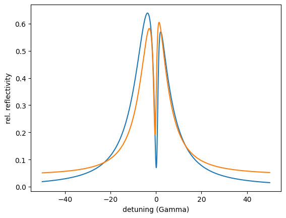
The Levenberg-Marquardt algorithm didn’t find a good solution, so let’s try another local algorithm.
# let's try a local gradient-free algorithm
opt.options.method = "Subplex"

opt.SetInitialVars()

opt()

plt.plot(detuning_reference, intensity_reference)
plt.plot(detuning_reference, energy_spectrum.result)
plt.xlabel('detuning (Gamma)')
plt.ylabel('rel. reflectivity')
plt.show()
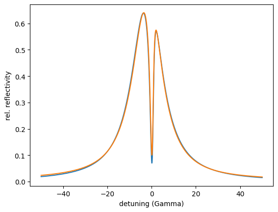
The Subplex algorithm did a much better job but its still not optimal. Go for a global algorithm.
# let's try a global algorithm
opt.options.method = "PagmoDiffEvol"

opt.SetInitialVars()

opt()

plt.plot(detuning_reference, intensity_reference)
plt.plot(detuning_reference, energy_spectrum.result)
plt.xlabel('detuning (Gamma)')
plt.ylabel('rel. reflectivity')
plt.show()
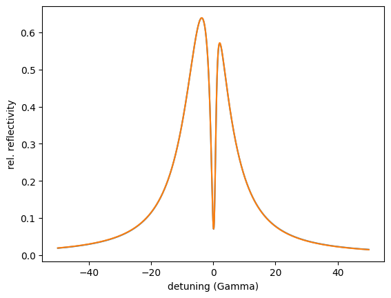
Finally, a good solution is found with the parameters
User residual start value: 10.330591

Starting optimizer with 2 provided measurement dependencies and 4 fit parameter(s).

  no. |                           id |       initial value |              min |              max
    0 |             Pt top thickness |                 3.2 |                0 |               10
    1 |                      B4C top |                   4 |                0 |               10
    2 |                      B4C mid |                   4 |                0 |               10
    3 |                      B4C top |                  16 |                0 |               20

Calling Pagmo solver with optimizer method PagmoDiffEvol

  population: 50
  iterations: 100

  cost = 9.499292e-04

Calling ceres solver with optimizer method LevMar

Ceres Solver Report: Iterations: 7, Initial cost: 1.804731e-06, Final cost: 1.804731e-06, Termination: CONVERGENCE

Optimizer finished with 4 fit parameter(s):

  no. |                           id |           fit value |       initial value |              min |              max
    0 |             Pt top thickness |             3.22195 |                 3.2 |                0 |               10
    1 |                      B4C top |             8.53259 |                   4 |                0 |               10
    2 |                      B4C mid |             5.50449 |                   4 |                0 |               10
    3 |                      B4C top |             15.0454 |                  16 |                0 |               20

Optimized user residual from 10.3306 to 0.00189986
The fit values are exactly the ones used to create the reference spectrum. At the end we also want to see the field intensity inside the sample.
# calcualte field intensity inside the sample
field_int = nx.FieldIntensity(sample = cavity,
                              energy = nx.moessbauer.Fe57.energy,
                              points = 1001)

depth, int = field_int()

plt.plot(depth, int)

# add lines and labels
axes = plt.gca()
y_min, y_max = axes.get_ylim()
plt.vlines(cavity.Interfaces(), y_min, y_max, colors='g', linestyles='dashed')
for id, location in zip(cavity.Ids(), np.array(cavity.Interfaces()) + 0.5):
    plt.text(location, y_max, id, fontsize = 10)
    y_max = y_max - 0.5

plt.xlabel('depth (nm)')
plt.ylabel('relative intensity')
plt.show()
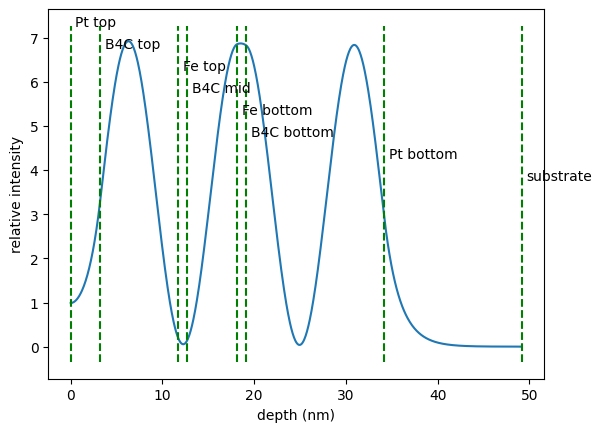
The two resonant iron layers are now in the node and antinode of the field.
Notebooks
fit global - nb_fit_global.ipynb.
fit errors - nb_fit_errors.ipynb.
fit multiple moessbauer - nb_fit_multiple_moessbauer.ipynb.
scipy optimize - nb_scipy_optimize.ipynb.
fit equality constraint - nb_fit_equality_constraint.ipynb.
fit external variable Bloch - nb_fit_external_variable_Bloch.ipynb.
fit inequality constraint - nb_fit_inequality_constraint.ipynb.
optimizer simple - nb_optimizer_simple.ipynb.
optimizer cavity - nb_optimizer_cavity.ipynb.
optimizer cavity multimodes - nb_optimizer_cavity_multimodes.ipynb.
optimizer spectrum - nb_optimizer_spectrum.ipynb.
Please have a look to the API Reference for more information.