Conuss Object
A ConussObject is an object in the beam path that is created from the .rof, which is calculated by the CONUSS module kref.
This class is implemented to put a diffraction object into the beam as long it is not available in Nexus directly.
Especially useful for Sychrotron Moessbauer Source (SMS) experiments to obtain the correct output field of the source.
The following parameters are Var objects and can be fit:
angle
divergence
A conuss object load data from a .rof file.
In the in_kref you can set the specific parameters for the calculation in CONUSS.
Most importantly for Nexus you define the parameter (9) energy range (gamma) :: E N_E and (10) angle range (microrad) :: X Y N_A.
E defines the energy range and the optional parameter N_E the number of points.
This is the energy grid on which the scattering matrices are calculated.
X and Y define the angular range and N_A the number of angles for which the scattering matrix is calculated.
Nexus then loads the N_A energy dependent scattering matrices.
It also extracts the electronic scattering contribution.
A ConussObject can only be created when a proper file_name is given.
Here, we load default.rof created by kref with the file in_kref.
It contains energy-dependent scattering matrices with 4001 grid points for 101 angles.
For calculations of energy or time spectra, the object behaves as a if a distribution with 101 points is given.
The set ditribution_points used for the thickness and divergence distributions are not changed.
Only the CONUSS object takes the number of points from the .rof file.
Do not wonder when fitting is slower with Nexus as with CONUSS for CONUSS objects.
The scattering matrices from CONUSS have to be interpolated to fit to the detuning grid of Nexus.
import nexus as nx
import numpy as np
import matplotlib.pyplot as plt

# create ConussObject from kref output file

# the two Var are used for all calculations and for fitting
ang = nx.Var(30e-6, min = 0, max = 100e-6, fit = True, id = "angle")
div = nx.Var(15e-6, min = 0, max = 50e-6, fit = True, id = "divergence")

co = nx.ConussObject(file_name = 'default.rof', angle = ang, divergence = div, id = "my conuss object")

# print the object
print(co)
The object print will show
ConussObject:
  .id: my conuss object
  .file_name: default.rof
  .angles: [-1.0e-04 -9.8e-05 -9.6e-05 -9.4e-05 -9.2e-05 -9.0e-05 -8.8e-05 -8.6e-05
 -8.4e-05 -8.2e-05 -8.0e-05 -7.8e-05 -7.6e-05 -7.4e-05 -7.2e-05 -7.0e-05
 -6.8e-05 -6.6e-05 -6.4e-05 -6.2e-05 -6.0e-05 -5.8e-05 -5.6e-05 -5.4e-05
 -5.2e-05 -5.0e-05 -4.8e-05 -4.6e-05 -4.4e-05 -4.2e-05 -4.0e-05 -3.8e-05
 -3.6e-05 -3.4e-05 -3.2e-05 -3.0e-05 -2.8e-05 -2.6e-05 -2.4e-05 -2.2e-05
 -2.0e-05 -1.8e-05 -1.6e-05 -1.4e-05 -1.2e-05 -1.0e-05 -8.0e-06 -6.0e-06
 -4.0e-06 -2.0e-06  0.0e+00  2.0e-06  4.0e-06  6.0e-06  8.0e-06  1.0e-05
  1.2e-05  1.4e-05  1.6e-05  1.8e-05  2.0e-05  2.2e-05  2.4e-05  2.6e-05
  2.8e-05  3.0e-05  3.2e-05  3.4e-05  3.6e-05  3.8e-05  4.0e-05  4.2e-05
  4.4e-05  4.6e-05  4.8e-05  5.0e-05  5.2e-05  5.4e-05  5.6e-05  5.8e-05
  6.0e-05  6.2e-05  6.4e-05  6.6e-05  6.8e-05  7.0e-05  7.2e-05  7.4e-05
  7.6e-05  7.8e-05  8.0e-05  8.2e-05  8.4e-05  8.6e-05  8.8e-05  9.0e-05
  9.2e-05  9.4e-05  9.6e-05  9.8e-05  1.0e-04]
  .detuning: [-300.   -299.85 -299.7  ...  299.7   299.85  300.  ]
  .angle: Var.value = 3e-05, .min = 0.0, .max = 0.0001, .fit: True, .id: angle
  .divergecne: Var.value = 1.5e-05, .min = 0.0, .max = 5e-05, .fit: True, .id: divergence
The object hold a couple of additional information saved in the co.object_info dict.
# print all additional object information from the co.object_info.
co.ObjectInfo()

# get single quantity from co.object_info dict
print("\n", co.object_info["energy start"])
header :  b'calculation ID: [**.00.92-**:00:**] -- project: FeBO3 003 reflection     <==57Fe{0.20}B{0.20}O{0.60}                                                                                                                                                                                '
Miller indices of reflection :  (0.0, 0.0, 3.0)
surface normal Bragg :  (0.0, 0.0, 1.0)
angle btw surface and netplanes :  0.0
conversion :  10.306486718230305
angle btw surface normal and incident x-ray :  1.6587349200228163
angle btw projection of incident x-ray k_in onto the surface and a reference vector :  1.570796326794896
angle btw surface normal and reflected x-ray :  1.4828577335669766
angle btw projection of reflected x-ray onto the surface and a reference vector :  1.570796326794896
Bragg angle :  0.08793859322791986
energy start :  -300.0
energy step :  0.15
energy number of points :  4001
angle minimum :  -9.999999999999999e-05
thickness step :  2e-06
angle number of points :  101
crystal thickness :  2.4999999999999998e-05
half lifetime :  9.781000000000001e-08
abundance :  0.95
mode :  b'Bragg reflection        '

 -300.0
To obtain the detuning grid used in CONUSS or the angles use
print(np.arrays(co.detuning))

print(np.array(co.angles))
[-300.   -299.85 -299.7  ...  299.7   299.85  300.  ]

[-1.0e-04 -9.8e-05 -9.6e-05 -9.4e-05 -9.2e-05 -9.0e-05 -8.8e-05 -8.6e-05
 -8.4e-05 -8.2e-05 -8.0e-05 -7.8e-05 -7.6e-05 -7.4e-05 -7.2e-05 -7.0e-05
 -6.8e-05 -6.6e-05 -6.4e-05 -6.2e-05 -6.0e-05 -5.8e-05 -5.6e-05 -5.4e-05
 -5.2e-05 -5.0e-05 -4.8e-05 -4.6e-05 -4.4e-05 -4.2e-05 -4.0e-05 -3.8e-05
 -3.6e-05 -3.4e-05 -3.2e-05 -3.0e-05 -2.8e-05 -2.6e-05 -2.4e-05 -2.2e-05
 -2.0e-05 -1.8e-05 -1.6e-05 -1.4e-05 -1.2e-05 -1.0e-05 -8.0e-06 -6.0e-06
 -4.0e-06 -2.0e-06  0.0e+00  2.0e-06  4.0e-06  6.0e-06  8.0e-06  1.0e-05
  1.2e-05  1.4e-05  1.6e-05  1.8e-05  2.0e-05  2.2e-05  2.4e-05  2.6e-05
  2.8e-05  3.0e-05  3.2e-05  3.4e-05  3.6e-05  3.8e-05  4.0e-05  4.2e-05
  4.4e-05  4.6e-05  4.8e-05  5.0e-05  5.2e-05  5.4e-05  5.6e-05  5.8e-05
  6.0e-05  6.2e-05  6.4e-05  6.6e-05  6.8e-05  7.0e-05  7.2e-05  7.4e-05
  7.6e-05  7.8e-05  8.0e-05  8.2e-05  8.4e-05  8.6e-05  8.8e-05  9.0e-05
  9.2e-05  9.4e-05  9.6e-05  9.8e-05  1.0e-04]
Amplitudes of a CONUSS object
In order to calculate amplitude properties, one has to select a scattering factors or object matrix at a certain index.
# angle at index 5
print(co.angles[5])

print(co.ScatteringFactorAtIndex(5))

print(np.squeeze(co.ObjectMatrixAtIndex(5)))

# or obtain an interpolated scattering matrix via
new_detuning = np.linspace(-200, 200, 1001)

print(np.squeeze(co.ObjectMatrixAtIndex(5, detuning=new_detuning)))
This code will only extract the values of the CONUSS object.
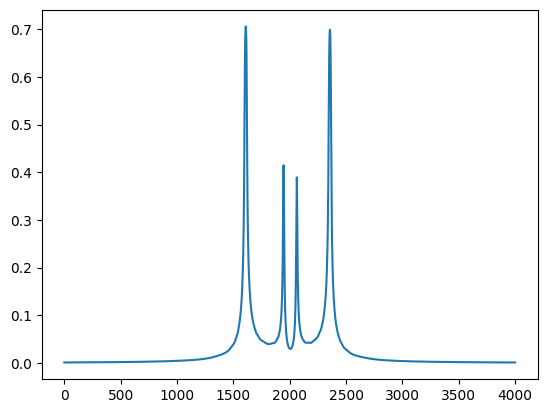
In order to calculate amplitude properties in an experiment you have to set the scattering factor and object matrix to be used. On default it is the central point of the grid - the index 50 in this example.
plt.plot(np.abs(np.array(co.ObjectMatrix())[:,1,0]))
plt.show()
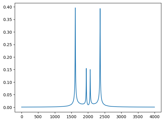
You can change this behavior by
co.SetPropertiesAtIndex(2)
print(co.angles[2])

plt.plot(np.abs(np.array(co.ObjectMatrix())[:,1,0]))
plt.show()
To obtain the angle of the index -9.6e-5 and the following plot
Note
In order to calculate object properties, always set the appropriate object matrix to the correct index.
When you set the CONUSS object properties like this, it is used for all amplitude calcualtions.
Notebooks
Download the conuss object notebook here nb_conuss_object.ipynb.
Please have a look to the API Reference for more information.