Hyperfine parameter distributions

Hyperfine parameters can be distributed over a range of magnitudes or angles. In order not to set a new Hyperfine for each point in a distribution manually, Nexus allows to define distributions for hyperfine parameters.

Distributions that act on a single parameter of the hyperfine object are introduced via the Distribution class. Nexus has predefined distributions implemented in the library lib.distribution, like Gaussian or Lorentzian and many more.

The Hyperfine class has two special methods for random angular distributions in 2D or 3D. These distributions require special treatment. One option is to set the Hyperfine.isotropic parameter. It is an analytical implementation of 3D angular distributions where both, the hyperfine field and the quadrupole splitting, are randomly distributed in 3D.

In case you want

• any kind of 2D angular distribution

• a 3D distribution acting on only the magnetic field or the quadrupole splitting

use the Hyperfine.SetRandomDistribution() method.

Note

Although a lib.distribution.Random class exists, do not use this to emulate 2D or 3D angular distributions. Two random distributions of two angles do not give a real random distribution of the angles! Only use Hyperfine.SetRandomDistribution() or Hyperfine.isotropic for random angular 2D and 3D angular distributions.

A Distribution object defines an array of delta values and the corresponding weight of the delta value. The delta values serve as an absolute difference to the target parameter. Most of the distributions do not need to know on which parameter they act. They just define the absolute differences to the target parameter they are applied to. This might seem a bit weird at the beginning but actually keeps the interface simple and flexible. A distribution can be applied to any target parameter. Internally, the delta values are just added to the parameter they are applied to.

Assume your target parameter has a value of X. The distribution has values from -Y to Y. Then the distribution will range from X-Y to X+Y. This is how most of the predefined distributions work. They calculate a range and are then applied to any target parameter you set them to.

The delta values can also serve as absolute values when the target parameter is zero. For a distribution with delta values from X to Y and a target parameter of 0, the distribution ranges from X to Y.

Note

An experiment should not have too many distributions. Each distribution point number multiplies with the previously set distribution points in a hyperfine site. For example, having three distributions with 30 points each will result in 27000 distribution points in total for the site. In this case the calculation of the transitions takes quite long. As a rule of thumb try to stay below 1000 distribution points per experiment for reasonable speeds.

Note

For 3D random distributions in both the magnetic field and the quadrupole splitting set Hyperfine.isotropic to True. This will results in considerable faster calculations than setting two 3D distributions via Hyperfine.SetRandomDistribution().

A simple distribution

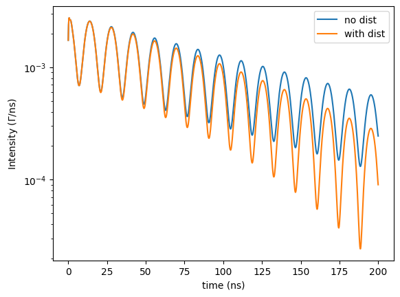
The following code should serve as the basis for the examples on distributions. Time spectra are calculated here, because effects due to distributions are better visualized in the quantum beat than in a Moessbauer spectrum.

# import packages
import nexus as nx
import numpy as np
import matplotlib.pyplot as plt

mat_Fe = nx.Material.Template(nx.lib.material.Fe)

layer_Fe = nx.Layer(id = "Fe",
                    material = mat_Fe,
                    thickness = 3000,  # in nanometer
                    roughness = 100)  # in nanometer

site = nx.Hyperfine(magnetic_field = 33,
                    magnetic_theta = 0,
                    magnetic_phi = 0)

mat_Fe.hyperfine_sites = [site]

sample = nx.Sample(layers = [layer_Fe])

beam  = nx.Beam()
beam.LinearSigma()

exp = nx.Experiment(beam = beam,
                    objects = [sample],
                    isotope = nx.moessbauer.Fe57)

time_spectrum = nx.TimeSpectrum(experiment = exp,
                                time_length = 200,
                                time_step = 0.2)

time_axis, intensity = time_spectrum.Calculate()

plt.semilogy(time_axis, intensity, label = 'no dist')

Now, a distribution of the magnetic field will be added. There are two different ways to do so. Either you define the distribution in the initializer or you can use a Set method to set it later.

So, either define the distribution before initializing the site

import nexus as nx
import numpy as np
import matplotlib.pyplot as plt

mat_Fe = nx.Material.Template(nx.lib.material.Fe)

layer_Fe = nx.Layer(id = "Fe",
                    material = mat_Fe,
                    thickness = 3000,  # in nanometer
                    roughness = 100)  # in nanometer

# definition of distribution
gauss_dist = nx.lib.distribution.Gaussian(points = 31,
                                          fwhm = 1)

# initializer definition
site = nx.Hyperfine(magnetic_field = 33,
                    magnetic_field_dist = gauss_dist,
                    magnetic_theta = 0,
                    magnetic_phi = 0)

mat_Fe.hyperfine_sites = [site]

sample = nx.Sample(layers = [layer_Fe])

or define it via a Set method on an existing Hyperfine object

# define a distribution from the library
# we have to define the number of points and the full width half maximum for a Gaussian distribution
gauss_dist = nx.lib.distribution.Gaussian(points = 31,
                                          fwhm = 1) # this can also be a fittable Var

# apply the distribution to the hyperfine parameter via set method
site.SetMagneticFieldDistribution(gauss_dist)

time_axis, intensity = time_spectrum.Calculate()

# plot the results
plt.semilogy(time_axis, intensity, label = 'with dist')

plt.xlabel('time (ns)')
plt.ylabel('Intensity ($\Gamma$/ns)')
plt.legend()
plt.show()

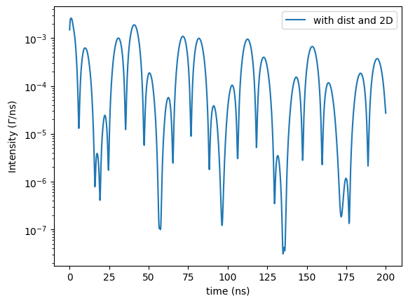
Let’s assume the magnetization has a random distribution in the \(\sigma-\pi\) plane (in the sample plane for forward scattering) in addition to the distribution in its amplitude.

# create a random distribution of the magnetic field angles
# the target can be either the magnetic field "mag" or the "efg"
# the type are either certain 2D distributions or a 3D distribution.
# random distributions can only be applied via a Set method.
site.SetRandomDistribution(target = "mag",
                           type  = "2Dsp", # random in the sigma-pi plane (sp)
                           points = 101)

plt.semilogy(*time_spectrum.Calculate(), label = 'with dist and 2D')

plt.xlabel('time (ns)')
plt.ylabel('Intensity ($\Gamma$/ns)')
plt.legend()
plt.show()

The Hyperfine has the attribute BareHyperfines. It holds all actual hyperfine site implementations generated via all distributions applied to the site. Those implementations are of type BareHyperfine, which only hold the bare hyperfine parameters. In order to see each actual hyperfine parameter due to distributions that belong to a hyperfine site you can use

for elem in site.BareHyperfines:
    print(elem)

Predefined Distributions

The easiest is to call one of the predefined distributions. It should fit most purposes. The lib.distribution library holds a lot of distribution types. For example,

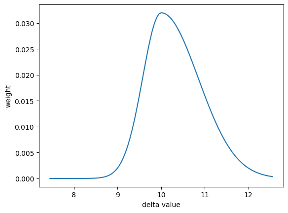
# define an asymmetric Gaussian distribution from the lib.distribution.
asym_gauss_dist = nx.lib.distribution.AsymmetricGaussian(
    points = 101,
    hwhm_low = nx.Var(value = 0.5, min = 0, max = 2, fit = True),
    hwhm_high = nx.Var(value = 1, min = 0, max = 2, fit = True))

# get the full width half maximum from the two set hwhm values
print("FWHM = {}".format(asym_gauss_dist.GetFWHM()))

# define a hyperfine site
site = nx.Hyperfine(magnetic_field = 10)

# define target parameter for the distribution
site.SetMagneticFieldDistribution(asym_gauss_dist)

# get the values and weight of the distribution
values, weight = site.GetMagneticFieldDistribution()

plt.plot(values, weight)
plt.xlabel('delta value')
plt.ylabel('weight')
plt.show()

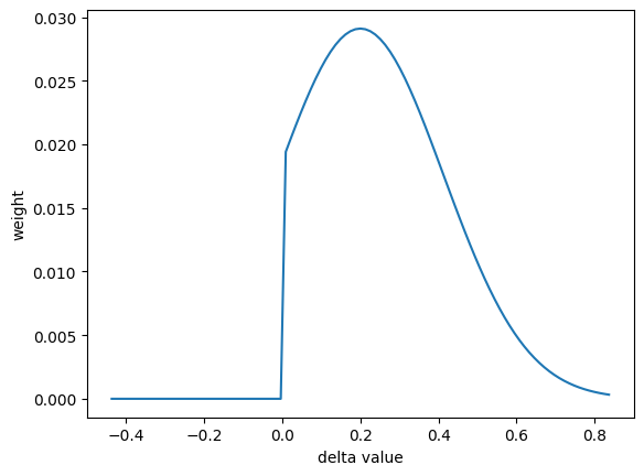
There are two predefined distributions that must know the target value. Those are PosGaussian and NegGaussian. These distributions must therefore only be applied to the specific target parameter that it takes as an argument.

site = nx.Hyperfine(quadrupole = 0.2)

# define a Gaussian distribution with only positive values from nexus.lib.distribution.
dist = nx.lib.distribution.PosGaussian(points = 101,
                                       fwhm = nx.Var(0.5, min = 0, max = 2, fit = True),
                                       target_var = site.quadrupole)

# only apply this dist to the quadrupole parameter
site.SetQuadrupoleDistribution(dist)

values, weight = site.GetQuadrupoleDistribution()

plt.plot(values, weight)
plt.xlabel('delta value')
plt.ylabel('weight')
plt.show()

Random Distributions

Note

This module is optimized in version 1.2.0. The function SetRandomDistribution(target, type, points, method, order)() now takes two more arguments, method and order parameters. The method attribute specifies the algorithm used, either random or model. The new random method is similar to the old random implementation, however, in the old version it used a true random sampling over the circles or spheres, which does not guarantee the correct spectrum. Now, random sampling based on vector parameter permutation and mirroring is used, which leads to better results. The new method model uses a group theoretical approach for optimized vector sampling. This method reduces the number of points necessary and is the default method. The given point number is not taken into account in this case. For 3D (spherical) distributions an order parameter can be specified, which determines the number of vector basis sets used. An order parameter of order=1 is sufficient for most cases.

The Hyperfine.SetRandomDistribution() method is used to set special multi-dimensional angular distributions. Those can be applied to either the magnetic hyperfine field or the quadrupole splitting. The distributions itself can be 3D or 2D, the latter lies in either of the planes spanned by the basis vectors given by \(\vec{\sigma}\), \(\vec{\pi}\) and \(\vec{k}\).

site = nx.Hyperfine(magnetic_field = 33)

# define a 2D random distribution of the magnetic field
# in the plane spanned by sigma and pi vectors ("sp")
site.SetRandomDistribution(target = "mag", type = "2Dsp", points = 401)

Note

The GetXXXDistribution() methods do not work for these random distributions.

Note

It is recommended to take at least 200 distribution points for magnetic random distributions. For EFG random distributions even larger values are recommended to about 1000 points.

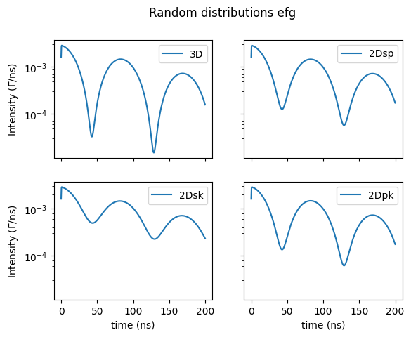
Here are the possible random distributions on the quadrupole splitting.

# import packages
import nexus as nx
import numpy as np
import matplotlib.pyplot as plt

mat_Fe = nx.Material.Template(nx.lib.material.Fe)

layer_Fe = nx.Layer(id = "Fe",
                    material = mat_Fe,
                    thickness = 3000,  # in nanometer
                    roughness = 100,  # in nanometer
                    )

site = nx.Hyperfine(quadrupole = 1.0)

mat_Fe.hyperfine_sites = [site]

sample = nx.Sample(layers = [layer_Fe])

beam  = nx.Beam()
beam.LinearSigma()

exp = nx.Experiment(beam = beam,
                    objects = [sample],
                    isotope = nx.moessbauer.Fe57
                    )

time_spectrum = nx.TimeSpectrum(experiment = exp,
                                time_length = 200,
                                time_step = 0.2,
                                max_detuning = 0)

fig, axs = plt.subplots(2,2, sharex=True, sharey=True)
fig.suptitle('Random distributions efg')

site.isotropic = True

axs[0,0].semilogy(*time_spectrum.Calculate(), label = 'isotropic', color = 'orange')

site.isotropic = False

points = 1001

site.SetRandomDistribution("efg", "3D", points)

# since v 1.2.0 it is valid to write
site.SetRandomDistribution("efg", "3D")

axs[0,0].semilogy(*time_spectrum.Calculate(), label = '3D', linestyle='dashed')
axs[0,0].legend()
axs[0,0].set_ylabel('Intensity ($\Gamma$/ns)')
axs[0,0].set_ylim([1e-5, 4e-3])

site.SetRandomDistribution("efg", "2Dsp", points)

axs[0,1].semilogy(*time_spectrum.Calculate(), label = '2Dsp')
axs[0,1].legend()

site.SetRandomDistribution("efg", "2Dsk", points)

axs[1,0].semilogy(*time_spectrum.Calculate(), label = '2Dsk')
axs[1,0].legend()
axs[1,0].set_xlabel('time (ns)')
axs[1,0].set_ylabel('Intensity ($\Gamma$/ns)')

site.SetRandomDistribution("efg", "2Dpk", points)

axs[1,1].semilogy(*time_spectrum.Calculate(), label = '2Dpk')
axs[1,1].legend()
axs[1,1].set_xlabel('time (ns)')

fig.show()

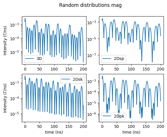
and the ones for the magnetic hyperfine field

# import packages
import nexus as nx
import numpy as np
import matplotlib.pyplot as plt

mat_Fe = nx.Material.Template(nx.lib.material.Fe)

layer_Fe = nx.Layer(id = "Fe",
                    material = mat_Fe,
                    thickness = 3000,  # in nanometer
                    roughness = 100,  # in nanometer
                    )

site = nx.Hyperfine(magnetic_field = 33)

mat_Fe.hyperfine_sites = [site]

sample = nx.Sample(layers = [layer_Fe])

beam  = nx.Beam()
beam.LinearSigma()

exp = nx.Experiment(beam = beam,
                    objects = [sample],
                    isotope = nx.moessbauer.Fe57)

time_spectrum = nx.TimeSpectrum(experiment = exp,
                                time_length = 200,
                                time_step = 0.2,
                                max_detuning = 0)

fig, axs = plt.subplots(2,2)
fig.suptitle('Random distributions mag')

site.isotropic = True

points = 401

axs[0,0].semilogy(*time_spectrum.Calculate(), label = 'isotropic', color = 'orange')

site.isotropic = False
site.SetRandomDistribution("mag", "3D", points)

# since v 1.2.0 it is valid to write
site.SetRandomDistribution("mag", "3D")

axs[0,0].semilogy(*time_spectrum.Calculate(), label = '3D', linestyle='dashed')
axs[0,0].legend()
axs[0,0].set_ylabel('Intensity ($\Gamma$/ns)')

site.SetRandomDistribution("mag", "2Dsp", points)


axs[0,1].semilogy(*time_spectrum.Calculate(), label = '2Dsp')
axs[0,1].legend()

site.SetRandomDistribution("mag", "2Dsk", points)

axs[1,0].semilogy(*time_spectrum.Calculate(), label = '2Dsk')
axs[1,0].legend()
axs[1,0].set_xlabel('time (ns)')
axs[1,0].set_ylabel('Intensity ($\Gamma$/ns)')

site.SetRandomDistribution("mag", "2Dpk", points)

axs[1,1].semilogy(*time_spectrum.Calculate(), label = '2Dpk')
axs[1,1].legend()
axs[1,1].set_xlabel('time (ns)')

fig.show()

Distribution from arrays

One can pass two arrays directly to a distribution. The first array is either the absolute difference or the absolute value of the hyperfine parameter. The second array is the weight.

With absolute differences

delta = np.linspace(-5, 5, 6)  # absolute differences to the target value
weight = np.linspace(0.1, 1, 6)  # some weight values

array_dist = nx.lib.distribution.Array(delta, weight)

site = nx.Hyperfine(magnetic_field = 30,  # distribution will range from 25 to 35
                    magnetic_theta = 90,
                    magnetic_phi = 30)

site.SetMagneticFieldDistribution(array_dist)

# Print all combinations applied to the site
print(site)

# print each parameter combination due to distributions stored in site.BareHyperfines
for elem in site.BareHyperfines:
    print(elem)

With absolute values

values = np.linspace(1, 30, 6)  # absolute values
weight = np.square(values)  # some dependence on values

array_dist = nx.lib.distribution.Array(values, weight)

array_dist.DistributionFunction()

site = nx.Hyperfine(magnetic_field = 0,  # zero because absolute values are assumed
                    magnetic_theta = 90,
                    magnetic_phi = 30
                    )

site.SetMagneticFieldDistribution(array_dist)

print(site)

for elem in site.BareHyperfines:
    print(elem)

Distribution from file

The distribution can be set with a file containing the distribution points and the weights, see distribution.txt.

31.2    0.3
32.2    0.5
33.2    0.8
34.2    0.3
35.2    0.1

The first column gives absolute differences or absolute values, e.g. the magnetic hyperfine field, and the second column the relative weights. Load the distribution with

# load a Distribution from a file
file_dist = nx.lib.distribution.File("distribution.txt")

site = nx.Hyperfine(magnetic_field = 0,  # zero because absolute field values are given
                    magnetic_theta = 90,
                    magnetic_phi = 30)

site.SetMagneticFieldDistribution(file_dist)

for elem in site.BareHyperfines:
    print(elem)

User defined distributions

User-defined distributions are advanced methods to create arbitrary distributions acting on a hyperfine site. The user must define a new distribution and provide the implementation of the mathematical function and the possible fit parameters. You define a child class inherited from the parent class Distribution. In this example, a Gaussian distribution is implemented by the user. The \(\sigma\) value of the Gaussian should be a fittable value.

class myGaussianDist(nx.Distribution):
    def __init__(self, points):
        # class inheritance
        super().__init__(points, "user defined Gaussian")
        # define a sigma class attribute
        self.sigma = nx.Var(value = 2, min = 0, max = 5, fit = True, id = "sigma")
        # register fit variables
        self.fit_varibales = [self.sigma]

This will define the new derived class myGaussianDist with a class instance attribute sigma of type Var that can be fit.

Next, implement the actual DistributionFunction(). The DistributionFunction() must set the delta values either by SetRange() or SetDelta() and the weight by SetWeight(). Those are the only requirements on this function. The SetRange() method sets the delta values symmetrically around zero over the given range, while the SetDelta() directly sets the values. Use numpy whenever possible for the function implementation for efficient calculations.

# define the distribution function
def DistributionFunction(self):

    # prevent division by zero in fitting
    if self.sigma.value == 0:
        self.sigma.value = 1e-299

    # set the delta values to a reasonable range
    x = self.SetRange(6 * self.sigma.value)

    # to process the x array with operators like +,-,*,/ in numpy, convert to numpy array
    x = np.array(x)

    # calculate the weight
    weight = np.exp(-1/2 * np.square(x) / np.square(self.sigma.value))

    # set the weight values
    self.SetWeight(weight)

The complete code for the distribution is

class myGaussianDist(nx.Distribution):
    def __init__(self, points):
        super().__init__(points, "user defined Gaussian")
        self.sigma = nx.Var(value = 2, min = 0, max = 5, fit = True, id = "sigma")
        self.fit_varibales = [self.sigma]

    def DistributionFunction(self):
        if self.sigma.value == 0:
            self.sigma.value = 1e-299
        x = self.SetRange(6 * self.sigma.value)
        weight = np.exp(-1/2 * np.square(x) / np.square(self.sigma.value))
        self.SetWeight(weight)

my_dist = myGaussianDist(points = 101)

In order to make your class more flexible and to use various instances of it, you can pass the sigma value in the __init__ method and define a class attribute which is given to the __init__ input.

class myGaussianDist(nx.Distribution):
    # put sigma to __init__ method
    def __init__(self, points, sigma):
        super().__init__(points, "user defined Gaussian")
        # set the class attribute to sigma
        self.sigma = sigma
        self.fit_varibales = [sigma]


    def DistributionFunction(self):
        if self.sigma.value == 0:
            self.sigma.value = 1e-299
        x = self.SetRange(6*self.sigma.value)
        weight = np.exp(-1/2*np.square(x)/(np.square(self.sigma.value)))
        self.SetWeight(weight)

my_dist = myGaussianDist(points = 101, sigma = nx.Var(1, min = 0, max = 7, fit = True))

sigma must be a Var object in this case. float assignment will not work. To do so you can change the code to:

class myGaussianDist(nx.Distribution):
    def __init__(self, points, sigma):
        super().__init__(points, "user defined Gaussian")
        self.sigma = sigma
        self.fit_varibales = [sigma]

    def DistributionFunction(self):
        if self.sigma == 0:
            self.sigma = 1e-299
        x = self.SetRange(6*self.sigma)
        weight = np.exp(-1/2*np.square(x)/(np.square(self.sigma)))
        self.SetWeight(weight)

my_dist = myGaussianDist(points = 101, sigma = 1)

But sigma will not be fittable in this case.

The user-defined functions do not need an analytical function to work. The lib.distribution.Array and lib.distribution.File distributions are also based on the Distribution parent class. For more advanced class definitions have a look to lib.distribution implementations.

Notebooks

distributions - nb_distributions.ipynb.