Data processing

The data module offers some functions to load, save and manipulate data or to extract information from data.

Loading data

Loading and saving data is basically done with numpy functions. Nexus offers two functions which load typical measured data sets.

For loading you can use nx.data.Load(). It has the following parameters

file_name: File to load (with relative path).
x_index: Column index in file for x axis data.
intensity_index: Column index in file for intensity data.
x_start: x data smaller than x_start are not considered.
x_stop: x data larger than x_stop are not considered.
intensity_threshold: intensity data <= intensity_threshold are not considered.

Loading a time spectrum from an ascii file in the measured time between 30ns and 150ns would look like this, when the first column gives the time in nanoseconds and the second column the intensity

import nexus as nx

time_data, intensity_data = nx.data.Load("my_filename",
                                         x_index = 0,
                                         intensity_index = 1,
                                         x_start = 30,
                                         x_stop = 150,
                                         intensity_threshold = None)

an additional threshold can be defined, to skip data below a certain intensity.

Saving data

Use the nx.data.Save() function, where you provide a filename and a list with the data arrays

# save some data arrays
num_points = 11

angles = np.linspace(0.1, 5, num_points)

intensity = np.random.rand(num_points)

nx.data.Save('example_file.txt', [angles, intensity])

Find Extrema

Note

New in version 1.0.2.

You can use the functions FindMinima() and FindMaxima() to extract the corresponding values of a data set.

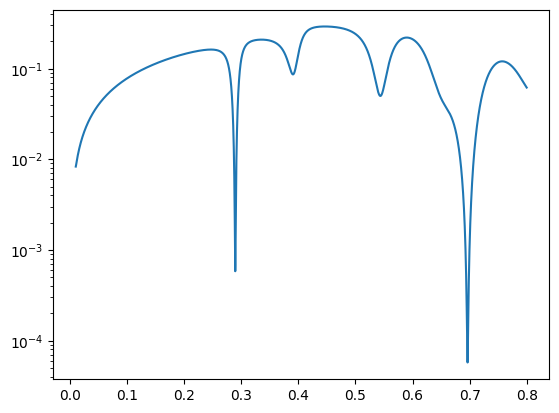
Let’s calculate the reflectivity of a cavity and find the minima.

import nexus as nx
import numpy as np
import matplotlib.pyplot as plt

lay_Pt_top = nx.Layer(id = "Pt top",
                material = nx.Material.Template(nx.lib.material.Pt),
                thickness = 2,
                roughness = 0.2)


lay_C = nx.Layer(id = "C",
                material = nx.Material.Template(nx.lib.material.C),
                thickness = 10,
                roughness = 0.3)

lay_Fe = nx.Layer(id = "Fe",
                  material = nx.Material.Template(nx.lib.material.Fe_enriched),
                  thickness = 1.5,
                  roughness = 0.35)

lay_Pt = nx.Layer(id = "Pt",
                material = nx.Material.Template(nx.lib.material.Pt),
                thickness = 15,
                roughness = 0.77)

lay_substrate = nx.Layer(id = "Si sub",
                material = nx.Material.Template(nx.lib.material.Si),
                thickness = nx.inf,
                roughness = 0.4
                )

sample1 = nx.Sample(id = "cavity",
                    layers = [lay_Pt_top,
                              lay_C,
                              lay_Fe,
                              lay_C,
                              lay_Pt,
                              lay_substrate],
                     geometry = "r",
                     length = 10,
                     roughness = "a")

beam  = nx.Beam(profile = "g", fwhm = 0.2)
beam.Unpolarized()

exp = nx.Experiment(beam = beam,
                    objects = [sample1],
                    id = "my exp")

angles = np.arange(0.01, 0.8, 0.0001)

reflectivity = nx.Reflectivity(experiment = exp,
                               sample = sample1,
                               energy = nx.lib.energy.CuKalpha,
                               angles = angles)

refl = reflectivity()

# the FindMinima function will return the x and y values as well as the indices
# all minima
print(nx.data.FindMinima(angles, refl))

# 1st minimum
print(nx.data.FindMinima(angles, refl, n=1))

plt.semilogy(angles, reflectivity())
plt.show()

(array([0.2894, 0.3905, 0.5436, 0.6963]), array([5.82265293e-04, 8.61527668e-02, 4.98477478e-02, 5.74210928e-05]), array([2794, 3805, 5336, 6863], dtype=int64))
(0.2893999999999983, 0.0005822652930938644, 2794)

Standard deviation

When you have loaded some data you might want to get the standard deviation for plotting an error estimate. Simply use

import nexus as nx

data_std = nx.data.HistogramStdDev(data)

It will calculate the square root of the data.

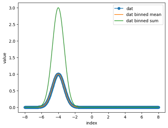
Binning

With the Binning() function is used for data binning/bucketing.

import nexus as nx
import numpy as np
import matplotlib.pyplot as plt

def gauss(x, offset):
  return np.exp(-1/2*(x-offset)**2/1*2)

axis = np.linspace(-8, 8, 1000)

dat = gauss(axis, -4)

bin_value = 3

end_point = False

bin_dat_mean = nx.data.Binning(dat, bin_value, "mean", end_point)

bin_dat_sum = nx.data.Binning(dat, bin_value, "sum", end_point)

axis_mean = nx.data.Binning(axis, bin_value, "mean", end_point)

plt.plot(axis, dat, marker = "o", label = "dat")
plt.plot(axis_mean, bin_dat_mean, label = "dat binned mean")
plt.plot(axis_mean, bin_dat_sum, label = "dat binned sum")

plt.xlabel('index')
plt.ylabel('value')
plt.legend()
plt.show()

Folding

A typical task is to fold data obtained from a Moessbauer drive. Nexus provides a function to manually select the folding point and two functions that use autocorrelation to do so.

nexus.data.Fold() to fold 1D data sets manually
nexus.data.AutoFold() to fold 1D data sets
nexus.data.AutoFold_2D() to fold 2D data sets

Changed in version 1.0.2.

The functions allow to flip either the left or right side of the spectrum.

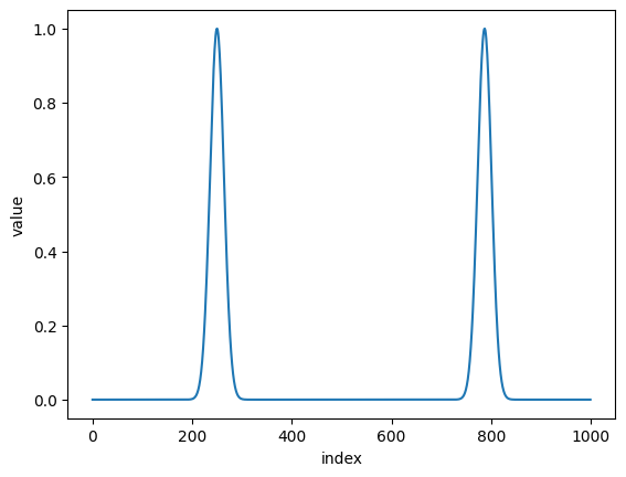
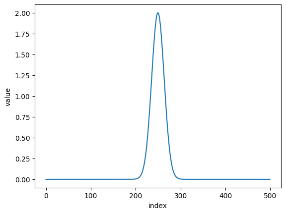
Let’s fold some data

import nexus as nx
import numpy as np
import matplotlib.pyplot as plt

def gauss(x, offset):
  return np.exp(-1/2*(x-offset)**2/0.1*2)

arr = np.linspace(-8, 8, 1000)

dat = gauss(arr, -4) + gauss(arr, 4.6)

plt.plot(dat)
plt.xlabel('index')
plt.ylabel('value')
plt.show()

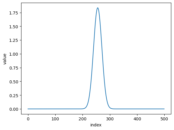
folded_dat = nx.data.Fold(dat, 512+37, flip = 'right')

plt.plot(folded_dat)
plt.xlabel('index')
plt.ylabel('value')
plt.show()

to get

or with the autocorrelation function

folded_dat, folding_point = nx.data.AutoFold(dat, flip = 'right')

print("folding_point {}".format(folding_point))

plt.plot(folded_dat)
plt.xlabel('index')
plt.ylabel('value')
plt.show()

folding_point 537

The 2D functions works similar along one axis. The function is mainly intended for energy time data sets.

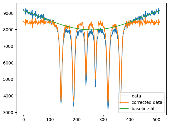
Baseline correction

Baseline correction might be needed in a measured spectrum. Nexus offers two functions to do so.

Be aware, that baseline correction changes the intensity of the lines.

For more options and other algorithms use the pybaselines package.

New in version 1.0.4.

Algorithms for baseline correction

Various algorithms can be used to find a good baseline correction.

aspls Adaptive Smoothness Penalized Least Squares.
mpls Morphological Penalized Least Squares.
asls Asymmetric Least Squares.
drlps Doubly Reweighted Penalized Least Squares.
arpls Asymmetrically Reweighted Penalized Least Squares.
iarpls Improved Asymmetrically Reweighted Penalized Least Squares.
amormol Iteratively averaging morphological and mollified baseline fit.

The lam value is the smoothing parameter. It has to be found for every algorithm and dataset by the user. A good procedure is to start with a low value (100) and then increase in an exponential manner (1e3, 1e4, …). At some point the curvature of the baseline changes. Then, reduce the values again and adjust.

import nexus as nx
import numpy as np
import matplotlib.pyplot as plt

data = np.loadtxt("example_baseline.txt")

new_data, baseline = nx.data.Baseline(data, lam = 1e9, algorithm='aspls', max_iter=100, tol=0.001)

plt.plot(data, label = "data")
plt.plot(new_data, label = "corrected data")
plt.plot(baseline, label = "baseline fit")

plt.legend()
plt.show()

Polynominal baseline correction

The polynominal baseline correction is up to an order specified by the user. Only data of the baseline should be used to find the correction. Therefore it uses masked data. Data between the two array indices left_point and right_point are not considered.

import nexus as nx
import numpy as np
import matplotlib.pyplot as plt

data = np.loadtxt("example_baseline.txt")

new_data, baseline = nx.data.BaselinePoly(data, left_point=100, right_point=400, poly_order=4)

plt.plot(data, label = "data")
plt.plot(new_data, label = "corrected data")
plt.plot(baseline, label = "baseline fit")

plt.legend()
plt.show()

Calibrating velocities

In order to calibrate the velocity of a data set use the functions CalibrateChannels(), CalibrateChannelsExperiment() or CalibrateChannelsAlphaFe(). CalibrateChannelsAlphaFe() returns a velocity grid calibrated to a theoretical \(\alpha\)-Fe spectrum. CalibrateChannelsExperiment() returns a velocity grid calibrated to user specified Experiment. CalibrateChannels() returns a velocity grid calibrated to a reference intensity and velocity.

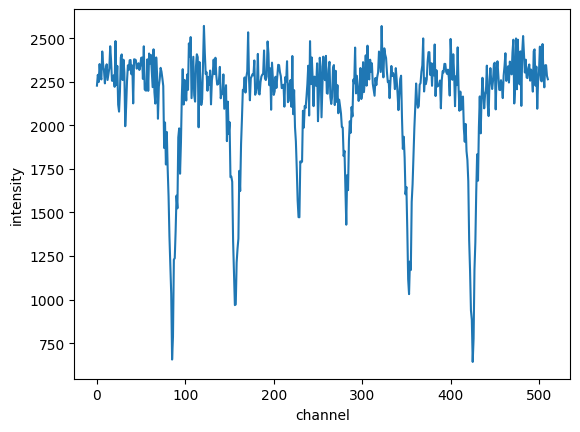
Here is an example Fe spectrum for which the calibrated velocity should be found Fe_alpha_spectrum. Let’s assume that the maximum velocity in the experiment was around 8 mm/s, we use an estimate of 8.6 mm/s.

import nexus as nx
import numpy as np
import matplotlib.pyplot as plt

intensity_exp = np.loadtxt("Fe_alpha_spectrum.txt")

plt.plot(intensity_exp)
plt.xlabel("channel")
plt.ylabel("intensity")
plt.show()

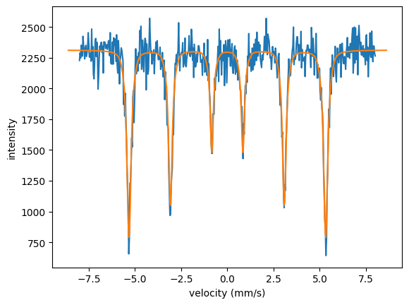
`CalibrateChannelsAlphaFe()`

The code

# the assumed maximum velocity was 8.6 mm/s and the sample thickness is 30 microns here.
v= 8.6
velocities, offset, scaling, vel_theo, int_theo = nx.data.CalibrateChannelsAlphaFe(
                                                    intensity = intensity_exp,
                                                    velocity= v,
                                                    thickness = 30e3,
                                                    Bhf = 33,
                                                    B_fwhm = 0.3,
                                                    emission = False,
                                                    mode = "constant",
                                                    shift = 0.0)

print("offset: {}".format(offset))
print("scaling: {}".format(scaling))
print("max velocity in experiment: {}".format(v*scaling))

# plot the experimental intensity vs the calibrated velocity
plt.plot(velocities, intensity_exp)
# plot the theory curved used for fitting
plt.plot(vel_theo, int_theo)
plt.xlabel("velocity (mm/s)")
plt.ylabel("intensity")
plt.show()

will result in

offset: -0.00027894605037020065
scaling: 0.9300171304868531
max velocity in experiment: 7.998147322186936

../../_images/Fe_spectrum_velocity_fit.png

As \(\alpha\)-Fe is a standard to calibrate the channels it has its own method. In case you want to use other calibration samples you can use the functions CalibrateChannelsExperiment() and CalibrateChannels().

`CalibrateChannelsExperiment()`

The same \(\alpha\)-Fe calibration can be achieved with the CalibrateChannelsExperiment() function and the Experiment class.

# setup an experiment used for the calibration
dist = nx.lib.distribution.Gaussian(points = 31,
                                    fwhm = 0.3)

site = nx.Hyperfine(magnetic_field = 33,
                    magnetic_field_dist = dist,
                    isotropic = True)

mat = nx.Material.Template(nx.lib.material.Fe)

mat.hyperfine_sites = [site]

layer = nx.Layer(thickness = 30e3,
                 material = mat)

sample = nx.Sample(layers = [layer])

beam = nx.Beam()
beam.Unpolarized()

exp = nx.Experiment(beam = beam,
                    objects = [sample],
                    isotope = nx.lib.moessbauer.Fe57)

# pass the experiment used for the calibration
v = 8.6
velocities, offset, scaling, vel_theo, int_theo = nx.data.CalibrateChannelsExperiment(
                                                    intensity = intensity_exp,
                                                    velocity = v,
                                                    experiment = exp,
                                                    emission = False,
                                                    mode = "constant",
                                                    shift = 0.0)

print("offset: {}".format(offset))
print("scaling: {}".format(scaling))
print("max velocity in experiment: {}".format(v*scaling))

plt.plot(velocities, intensity_exp)
plt.plot(vel_theo, int_theo)
plt.xlabel("velocity (mm/s)")
plt.ylabel("intensity")
plt.show()

`CalibrateChannels()`

Or use the CalibrateChannels() function and a pre-calculated Measurement by passing the intensity and velocity of the calculation

# setup and intensity calculation
dist = nx.lib.distribution.Gaussian(points = 31,
                                    fwhm = 0.3)

site = nx.Hyperfine(magnetic_field = 33,
                    magnetic_field_dist = dist,
                    isotropic = True)

mat = nx.Material.Template(nx.lib.material.Fe)

mat.hyperfine_sites = [site]

layer = nx.Layer(thickness = 30e3,
                 material = mat)

sample = nx.Sample(layers = [layer])

beam = nx.Beam()
beam.Unpolarized()

exp = nx.Experiment(beam = beam,
                    objects = [sample],
                    isotope = nx.lib.moessbauer.Fe57)

#assumed maximum detuning is 8.6 mm/s
vel_theory = np.linspace(-8.6, 8.6, len(intensity_exp))

spec = nx.MoessbauerSpectrum(experiment = exp,
                             velocity = vel_theory)

spec_theory = spec()

v = 8.6
velocities, offset, scaling, vel_theo, int_theo = nx.data.CalibrateChannels(
                                                    intensity = intensity_exp,
                                                    velocity = v,
                                                    intensity_reference = spec_theory,
                                                    velocity_reference = vel_theory,
                                                    mode = "constant",
                                                    shift = 0.0)

print("offset: {}".format(offset))
print("scaling: {}".format(scaling))
print("max velocity in experiment: {}".format(v*scaling))

plt.plot(velocities, intensity_exp)
plt.plot(vel_theo, int_theo)

plt.xlabel("velocity (mm/s)")
plt.ylabel("intensity")
plt.show()

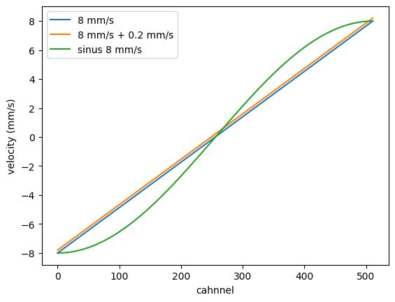
Simple velocity grid

You can also define a simple velocity grid by the function ChannelsToVelocity().

import nexus as nx
import numpy as np
import matplotlib.pyplot as plt

velocity = nx.data.ChannelsToVelocity(num_channels = 512, velocity = 8, mode = "constant")

plt.plot(velocity, label = "8 mm/s")

velocity = nx.data.ChannelsToVelocity(num_channels = 512, velocity = 8, offset = 0.2, mode = "constant")

plt.plot(velocity, label = "8 mm/s + 0.2 mm/s")

velocity = nx.data.ChannelsToVelocity(num_channels = 512, velocity = 8, mode = "sinus")

plt.plot(velocity, label = "sinus 8 mm/s")
plt.xlabel("cahnnel")
plt.ylabel("velocity (mm/s)")
plt.legend()
plt.show()