Hello Nexus
The Hello Nexus examples give a basic introduction to the calculation of Moessbauer spectra and time spectra in forward geometry. An example for the calculation of the electronic reflectivity and a simple fit example are given as well.
In order to use Nexus you have to import it to Python as any other package.
In the tutorial we use import nexus as nx, similar to the typical numpy import import numpy as np.
The basic tutorial will be kept as simple and clear as possible. For all optional parameters of the classes and methods have a look to the specific tutorials or the API Reference. In the tutorial on specific methods we will cover most of the optional parameters.
Note
It is recommended to use keywords arguments in all of Nexus functions and objects to keep the interface as clear as possible. This is done throughout the tutorial.
Moessbauer spectrum
The most basic Measurement is a Moessbauer spectrum, here a single iron foil is used.
The following code calculates a Moessbauer spectrum.
# import packages
import nexus as nx
import numpy as np
import matplotlib.pyplot as plt

iron = nx.Material.Template(nx.lib.material.Fe)

layer_Fe = nx.Layer(id = "Fe layer",
                    material = iron,
                    thickness = 3000)

site = nx.Hyperfine(magnetic_field = 33,
                    isotropic = True)

iron.hyperfine_sites = [site]

sample = nx.Sample(layers = [layer_Fe])

beam = nx.Beam(polarization = 0)

exp = nx.Experiment(beam = beam,
                    objects = [sample],
                    isotope = nx.lib.moessbauer.Fe57)

velocities = np.linspace(-10, 10, 512)

moessbauer_spectrum = nx.MoessbauerSpectrum(experiment = exp,
                                            velocity = velocities,
                                            id  = "my first spectrum")

intensity = moessbauer_spectrum.Calculate()

plt.plot(velocities, intensity)
plt.xlabel('velocity (mm/s)')
plt.ylabel('transmission')
plt.show()
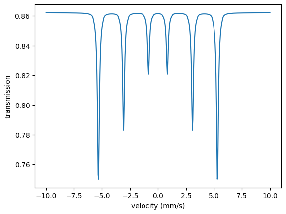
Et voila.
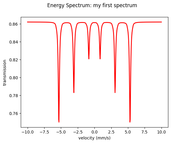
Note
New in version 1.0.3: added Plot() method for all measurements.
# to plot the velocities instead of detuning set velocity to True.
moessbauer_spectrum.Plot(velocity = True)
Let’s go through this example step by step.
First, the experiment has to be set up.
Start with a Sample:
# import packages
import nexus as nx
import numpy as np
import matplotlib.pyplot as plt

# define a sample with one layer and one set of hyperfine parameters

# the material is loaded from the nexus.lib.material library which hosts a lot of predefined materials
# the predefined Fe contains the isotope properties already
# The Material.Template method loads the material from the library properly.
iron = nx.Material.Template(nx.lib.material.Fe)

# look at all the material parameters of the iron pre-defined material
print(iron)

# create a layer
layer_Fe = nx.Layer(id = "Fe layer",  # this is an optional user defined string identifier.
                    material = iron,  # assign the material previously loaded
                    thickness = 3000)  # in nanometer

print(layer_Fe)

# define Hyperfine parameters
# only one set of parameters, called a site, is used here
# the hyperfine field of 33 T is assumed to be isotropically distributed.
# the Hyperfine site has much more parameters, e.g. the quadrupole splitting,
# but they are set to zero for now (the default value)
site = nx.Hyperfine(magnetic_field = 33,
                    isotropic = True)

# look at all the hyperfine parameters of the site
print(site)

# the class attribute you have set can be accessed directly
# here the magnetic field
print(site.magnetic_field)

# it will print the properties of a Var object.
# Nexus internally converts your input to the Var class type.
# don't care too much for now, it is important for fitting
# a Var object has the shown properties, which can be accessed
print(site.magnetic_field.value)

# set the materials hyperfine sites by a list
# you can put as many sites as you want to the list
iron.hyperfine_sites = [site]

# define the layers of the sample by a list
# you can define as many layers as you want
# the order in the list gives the layer order along the beam path
sample = nx.Sample(layers = [layer_Fe])

# print the sample
print(sample)
The prints will give information on the objects you created
Material
  .id: Fe
  .composition:  Fe 1.0
  .density (g/cm^3) Var.value = 7.874, .min = 0.0, .max = 7.874, .fit: False, .id:
  .isotope: 57-Fe
  .abundance Var.value = 0.02119, .min = 0.0, .max = 1.0, .fit: False, .id:
  .lamb_moessbauer Var.value = 0.796, .min = 0.0, .max = 1.0, .fit: False, .id:
    derived parameters:
    .total_number_density (1/m^3) = 8.487550450450646e+28
    .average_mole_mass (g/mole) = 55.868105434026994
    .isotope_number_density (1/m^3) = 1.7985119404504918e+27
    number of hyperfine sites 0

Layer
  .id: Fe layer
  .material.id: Fe
  .material.composition:  Fe 1.0,
  .material.density (g/cm^3) Var.value = 7.874, .min = 0.0, .max = 7.874, .fit: False, .id:
  .thickness (nm) Var.value = 3000.0, .min = 0.0, .max = inf, .fit: False, .id:
  .roughness (nm, sigma) Var.value = 0.0, .min = 0.0, .max = inf, .fit: False, .id:
  .thickness_fwhm (nm) Var.value = 0.0, .min = 0.0, .max = inf, .fit: False, .id:

Hyperfine .id:
  .weight =               1.0
  .isomer_shift =         0.0        dist points: 1
  .magnetic_field =       33.0       dist points: 1
  .magnetic_theta =       0.0        dist points: 1
  .magnetic_phi =         0.0        dist points: 1
  .quadrupole =           0.0        dist points: 1
  .quadrupole_alpha =     0.0        dist points: 1
  .quadrupole_beta =      0.0        dist points: 1
  .quadrupole_gamma =     0.0        dist points: 1
  .quadrupole_asymmetry = 0.0        dist points: 1
  .isotropic =            True       3D distribution in mag and efg. Random mag or efg distributions are ignored.
  random magnetic distribution: none         dist points: 1
  random quadrupole distribution: none       dist points: 1
  total number of distribution points: 1

Sample
  .id:
  .geometry: f
  .angle (deg) = 0.0
  .divergence (deg) = 0.0
  .length (mm) = 10.0
  .roughness (model): a
-------|------------------------|---------------|-------------|-------------|--------|-----------|----------|-------------|
 index |               Layer id | dens. (g/cm3) | thick. (nm) | rough. (nm) | abund. | LM factor | HI sites | dist points |
-------|------------------------|---------------|-------------|-------------|--------|-----------|----------|-------------|
     0 |               Fe layer |         7.874 |      3000.0 |         0.0 |0.02119 |     0.796 |        1 |           1 |
-------|------------------------|---------------|-------------|-------------|--------|-----------|----------|-------------|
Now the Experiment is set up.
# define a beam
# set polarization to zero for classical Moessbauer spectroscopy
beam = nx.Beam(polarization = 0)

# define the experiment
exp = nx.Experiment(beam = beam,
                    objects = [sample],                # a list of objects in the beam path
                    isotope = nx.lib.moessbauer.Fe57)  # define the isotope for calculation
                                                       # loaded from a pre-defined isotope in the library

print(exp)

# let's have a look to the isotope properties
print(exp.isotope)
The objects prints are
Experiment .id:
  .beam.id:
  .objects:
    index: 0, type: Sample, .id:

MoessbauerIsotope: 57-Fe
  .element = Fe
  .mass (u) = 56.9353933
  .spin_ground = 0.5
  .spin_excited = 1.5
  .energy (eV) = 14412.497
  .wavelength (m) = 8.602548e-11
  .kvector (1/m) = 7.303865e+10
  .lifetime (s) = 1.4111000000000002e-07
  .gamma (eV) = 4.664530911345758e-09
  .internal_conversion = 8.21
  .multipolarity = M1 (L = 1, lambda = 0)
  .mixing_ratio_E2M1 = 0.0
  .gfactor_ground = 0.18121
  .gfactor_excited = -0.10348
  .quadrupole_ground (barn) = 0.0
  .quadrupole_excited (barn) = 0.187
  .magnetic_moment_ground (eV/T) = 2.85627845959275e-09
  .magnetic_moment_excited (eV/T) = -4.8932348380110005e-09
  .nuclear_cross_section (converted to kbarn) = 2557.671207310153
Set up a MoessbauerSpectrum
# define a velocity range of the calculation
velocities = np.linspace(-10, 10, 512)  # in mm/s

# define the Moessbauer spectrum measurement object
moessbauer_spectrum = nx.MoessbauerSpectrum(experiment = exp,
                                            velocity = velocities,
                                            id  = "my first spectrum")

# calculate the Moessbauer spectrum from the object
# returns the intensity as a numpy array
intensity = moessbauer_spectrum.Calculate()

# plot the result
plt.plot(velocities, intensity)
plt.xlabel('velocity (mm/s)')
plt.ylabel('transmission')
plt.show()
That’s it.
SimpleSample
New in version 1.0.4.
A new SimpleSample class is available.
It creates a Sample with only one layer and material.
All needed instances are created automatically.
The example also could be generated by the following code.
# import packages
import nexus as nx
import numpy as np
import matplotlib.pyplot as plt

site = nx.Hyperfine(magnetic_field = 33,
                    isotropic = True)

sample = nx.SimpleSample(thickness=3000,
                       composition = [["Fe", 1]],
                       density = 7.874,
                       isotope = nx.lib.moessbauer.Fe57,
                       abundance = 0.02119,
                       lamb_moessbauer = 0.796,
                       hyperfine_sites = [site])

beam = nx.Beam(polarization = 0)

exp = nx.Experiment(beam = beam,
                    objects = [sample],
                    isotope = nx.lib.moessbauer.Fe57)

velocities = np.linspace(-10, 10, 512)

moessbauer_spectrum = nx.MoessbauerSpectrum(experiment = exp,
                                            velocity = velocities,
                                            id  = "my first spectrum")

moessbauer_spectrum.Calculate()

moessbauer_spectrum.Plot(velocity = True)
Time spectrum
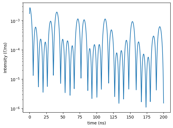
To calculate a time spectrum of the same experiment as before we just have to change the measurement to a time spectrum. So, everything up to the experiment is the same.
# define the time spectrum measurement object
time_spectrum = nx.TimeSpectrum(experiment = exp,
                                time_length = 200,  # in ns
                                time_step = 0.2)    # in ns

# calculate the time spectrum from the object
# a calculation can also be performed by the () operator instead of .Calculate()
# the time spectrum will return the time axis and the intensity
time_axis, intensity = time_spectrum()

plt.semilogy(time_axis, intensity)
plt.xlabel('time (ns)')
plt.ylabel('Intensity ($\Gamma$/ns)')
plt.show()
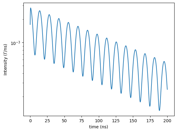
However, in a nuclear resonant scattering experiment the synchrotron beam is polarized. Let’s also assume that a magnetic field is applied to saturate the magnetization and the hyperfine field.
# the synchrotron beam is linearly polarized along sigma direction
beam.LinearSigma()

# and we assume that an external magnetic field aligns the hyperfine field along the beam direction
# so the hyperfine field is not longer isotropically distributed
site.isotropic = False
# the polar angle theta is defined from the photon k vector direction
site.magnetic_theta = 0
# the azimuthal angle phi is defined in the sigma pi plane starting from the sigma direction
site.magnetic_phi = 0

time_axis, intensity = time_spectrum()

plt.semilogy(time_axis, intensity)
plt.xlabel('time (ns)')
plt.ylabel('Intensity ($\Gamma$/ns)')
plt.show()
Fitting
Data fitting is one of the most important functions of Nexus. Nexus offers several methods, like gradient based and gradient free or local and global fit algorithms.
Let’s try to fit a simulated Moessbauer spectrum where some Gaussian noise has been added and the scaling has been changed.
The data set is that of an iron foil as calculated before as example_spectrum.
The first column gives the velocity in units of mm/s and the second one the counts.
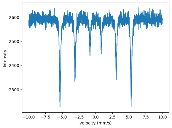
Let’s load the data with numpy and plot them.
import nexus as nx
import numpy as np
import matplotlib.pyplot as plt

data = np.loadtxt('example_spectrum.txt')

velocity_experiment = data[:,0]
intensity_experiment = data[:,1]

plt.plot(velocity_experiment, intensity_experiment)
plt.xlabel('velocity (mm/s)')
plt.ylabel('rel. transmission')
plt.show()
To fit a measured data set, start as before.
Define your Experiment and the Measurement.
Here, we assume some hyperfine parameters, let’s say a magnetically split line in a magnetic field of 31 T, which is randomly distributed in space.
All fittable parameters in Nexus are of type Var - a fit variable.
Although floats have been assigned before, they are internally initialized as Var objects by Nexus.
Almost all numerical values of classes in Nexus are of type Var, except parameters of the MoessbauerIsotope class.
In order to fit a parameter, the fit argument of the Var has to be set to True.
We also give some boundaries for fitting, a minimum and maximum value.
Therefore, initialize the magnetic field as a Var object directly.
Also, provide a unique id in order to identify the Vars in the output of the fit routines.
# Var objects can be defined directly in the class initialization.
site = nx.Hyperfine(magnetic_field = nx.Var(value = 31, min = 25, max = 35, fit = True, id = "magnetic field"),
                    isotropic = True)

# the Var object of the site is referenced like this
print(site.magnetic_field)

# Alternatively, you can also define the Var object directly
mag_field = nx.Var(value = 28, min = 25, max = 35, fit = True, id = "magnetic field")

site = nx.Hyperfine(magnetic_field = mag_field,
                    isotropic = True)

print(mag_field)

# continue with a material
mat_Fe = nx.Material.Template(nx.lib.material.Fe)

mat_Fe.hyperfine_sites = [site]

layer_Fe = nx.Layer(id = "Fe",
                    material = mat_Fe,
                    thickness = 3000)  # in nanometer

sample = nx.Sample(layers = [layer_Fe])

beam = nx.Beam()

# set the beam polarization via a class method
beam.Unpolarized()

exp = nx.Experiment(beam = beam,
                    objects = [sample],
                    isotope = nx.lib.moessbauer.Fe57)
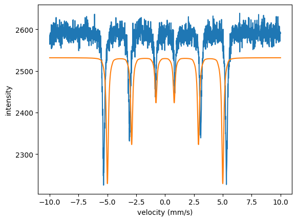
Create a MoessbauerSpectrum and pass the data to be fit as well.
Measured data should always be provided in the Measurement initialization.
This ensures that the grid for the calculation and the measured data always fit together.
spectrum = nx.MoessbauerSpectrum(experiment = exp,
                                 velocity = velocity_experiment,  # the measured velocity
                                 intensity_data = intensity_experiment)  # the measured intensity to be fit

# calculate the intensity from the assumed model
intensity = spectrum.Calculate()

# plot both the model and the measured data
plt.plot(velocity_experiment, intensity_experiment)
plt.plot(velocity_experiment, intensity)
plt.xlabel('velocity (mm/s)')
plt.ylabel('intensity')
plt.show()
Or use spectrum.Plot(velocity = True) for plotting.
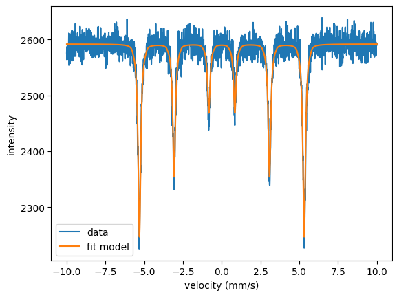
The model and the data do not fit, the intensity is not correct and the magnetic field value is off.
Nexus will adjust all those values while fitting.
A Fit object is used to fit data sets. The Measurements to be fit has to be specified.
# create a fit object with a list of measurements to be fit in parallel.
fit = nx.Fit(measurements = [spectrum])

# run the fit
fit.Evaluate()
In jupyter, you will get output from the Fit module that should look like this.
Starting fit with 1 measurement data set(s) and 2 fit parameter(s).

  no. |                           id |       initial value |              min |              max
    0 |                   ES scaling |             2638.74 |                0 |           263874
    1 |               magnetic field |                  31 |               25 |               35

Calling ceres solver with fit method LevMar

Ceres Solver Report: Iterations: 6, Initial cost: 1.032466e+04, Final cost: 2.201971e+01, Termination: CONVERGENCE

Fit performed with 2 fit parameter(s).

  no. |                           id |           fit value |       initial value |              min |              max
    0 |                   ES scaling |             3000.41 |             2638.74 |                0 |           263874
    1 |               magnetic field |             32.9482 |                  31 |               25 |               35

total cost = 2.201971e+01

cost for each FitMeasurement is:

  no. |                           id |                cost |                   %
    0 |                              |        2.201971e+01 |             100.000
Note
In the command line additional output by the Fit module is provided.
Some output of this module is not parsed to an interactive interpreter, like IDLE or jupyter.
That information is not really needed by the user but can help in order to optimize fitting, see that the fit is running and estimate how long it will take.
In the first block Nexus informs you about its initial configuration, what the fit parameters are and which method is used.
There is the ES scaling (energy spectrum scaling) value that pops up but it has not been initialized by us as a fit object.
It is the scaling factor for the theory to fit the data and automatically added by Nexus as long as it is not further specified by the user in the Measurement.
In the standard setting Nexus is using the Levenberg-Marquardt algorithm as implemented by the [Ceres] solver. It is a reliable local and gradient-based algorithm which works well if there are not many local minima in the hyperspace of the fit parameters or when your guess is already close to the solution.
Then, the fit results are given.
The \(cost\) is an indicator of the goodness of a fit (see Fitting and Optimization).
Then, the fitted values are given.
Nexus also shows the contribution of each Measurement to the overall \(cost\).
This information is important for mulit-measurement fitting.
You can see that the intensity scaling went from Nexus inital guess of 2638.74 to 3000 and the magnetic field from 31 to 33.
Note that in Nexus a fit does not only mean that the fitted values are printed.
The values are actually changed internally.
Thus after the fit, the site.magnetic_field.value is now 33.
Let’s check that and plot the data.
# print the fitted value
print(site.magnetic_field.value)

# plot the data
# after a calculation or fit, the methods output can also be accessed via the .result attribute of the measurement
# so you don't have to recalculate the output via spectrum.Calcualte()
plt.plot(velocity_experiment, spectrum.result , label = 'fit model') # our fit model
plt.plot(velocity_experiment, intensity_experiment, label = 'data')  # the 'measured' data

plt.legend()
plt.xlabel('velocity (mm/s)')
plt.ylabel('Intensity')
plt.show()

The model is fit to the data.
Or use spectrum.Plot(velocity = True) for plotting.
Now let’s use another method, a special version of the differential evolution algorithm as implemented by the [Pagmo] package. It is a global gradient-free algorithm. In order to do so we don’t have to do much.
# we set all fit parameters back to their initial start values before the fit.
# there is a special method for this
fit.SetInitialVars()

# change the fit method in the fit options
fit.options.method = "PagmoDiffEvol"

fit.Evaluate()
Again in jupyter, the output should look like the following
Starting fit with 1 measurement data set(s) and 2 fit parameter(s).

  no. |                           id |       initial value |              min |              max
    0 |                   ES scaling |             2638.74 |                0 |           263874
    1 |               magnetic field |                  31 |               25 |               35

Calling Pagmo solver with fit method PagmoDiffEvol

  population: 30
  iterations: 100

  cost = 2.136686e+01

Calling ceres solver with fit method LevMar

Ceres Solver Report: Iterations: 1, Initial cost: 2.136686e+01, Final cost: 2.136686e+01, Termination: CONVERGENCE

Fit performed with 2 fit parameter(s).

  no. |                           id |           fit value |       initial value |              min |              max
    0 |                   ES scaling |             3000.48 |             2638.74 |                0 |           263874
    1 |               magnetic field |             32.9955 |                  31 |               25 |               35

  total cost = 2.136686e+01

cost for each FitMeasurement is:

  no. |                           id |                cost |                   %
    0 |                              |        2.136686e+01 |             100.000
Nexus has used the Pagmos Differential Evolution algorithm.
It is automatically followed by a local algorithm to do the local optimization of the best result found by the global algorithm.
The standard is the LevMar algorithm again.
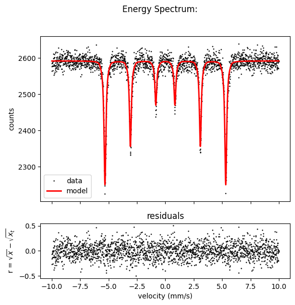
Let’s plot the result.
# and plot the data
plt.plot(velocity_experiment, intensity_experiment, label = 'data')  # the 'measured' data
plt.plot(velocity_experiment, spectrum.result , label = 'fit model') # our fit model
plt.legend()
plt.xlabel('velocity (mm/s)')
plt.ylabel('intensity')
plt.show()
Again, we find the same values and the choice of the algorithm didn’t changed our result.
The example is quite trivial but for more complex fit scenarios the choice of the algorithm can strongly influence the result.
These two algorithms should be your first choice for local or global fitting, respectively.
There are a lot more algorithms implemented which you can all find in the API Reference under Fit.OptimizerOptions.
Reflectivity
A reflectivity does not take into account nuclear scattering, it calculates electronic scattering only.
So, we do not need to define hyperfine parameters.
To measure a nuclear reflectivity (either in energy or the time domain) there are special methods.
In order to calculate a reflectivity of a thin film system we have to define a sample. Here, an iron film on a silicon substrate.
This time we define the material as well and do not use the lib.material.
import nexus as nx
import numpy as np
import matplotlib.pyplot as plt

# iron layer
# no isotope defined, only electronic calculations
material_Fe = nx.Material(id = "iron",
                          composition = [["Fe", 1]],
                          density = 7.874)

layer_Fe = nx.Layer(id = "Fe",
                    material = material_Fe,
                    thickness = 10,   # nm
                    roughness = 0.4)  # nm

# silicon substrate
substrate_Si = nx.Layer(id = "Si substrate",
                        material = nx.Material.Template(nx.lib.material.Si),
                        thickness = nx.inf,      # set the substrate to infinite thickness
                        roughness = 0.3)

# define sample
# in grazing incidence the beam profile and the sample length get important
sample = nx.Sample(layers = [layer_Fe, substrate_Si],  # define layers from top to bottom
                   geometry = "r",                     # set the sample geometry to reflectivity
                   length = 10)                        # in mm
Now, the experiment can be set up.
# standard initialization of a beam is linear sigma polarization
# the polarization properties are not accounted for in electronic calculations
# in grazing incidence the beam profile and the size of the beam are important
beam  = nx.Beam(profile = 'g',  # Gaussian beam profile
                fwhm = 0.2)     # FWHM of the beam in the scattering plane, in mm

exp = nx.Experiment(beam = beam,
                    objects = [sample])
Create the reflectivity measurement of the experiment.
# reflectivity measurement

# define the angles for the calculations
angles = np.arange(0.001, 6, 0.001)

# create reflectivity object
# because in every experiment there can be a lot of objects you have to specify the sample for which the angles are changed
# this is done by the sample keyword
reflectivity = nx.Reflectivity(experiment = exp,
                               sample = sample,  # object for the reflectivity calculation
                               energy = nx.lib.energy.CuKalpha,  # Cu K alpha line
                               angles = angles)

# the standard setting for a sample in grazing incidence reflection
# are with an analytical roughness model
plt.semilogy(angles, reflectivity(), label = 'with roughness')

# calculate again without taking sample roughness into account
sample.roughness = "n"

plt.semilogy(angles, reflectivity(), label = 'no roughness')
plt.legend()
plt.xlabel('angle (deg)')
plt.ylabel('reflectivity')
plt.show()
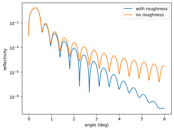
Please note that the theoretical calculation of roughness is not straight forward and brings a lot of complications to the theory. In order to get the best results the physical roughness should be low.
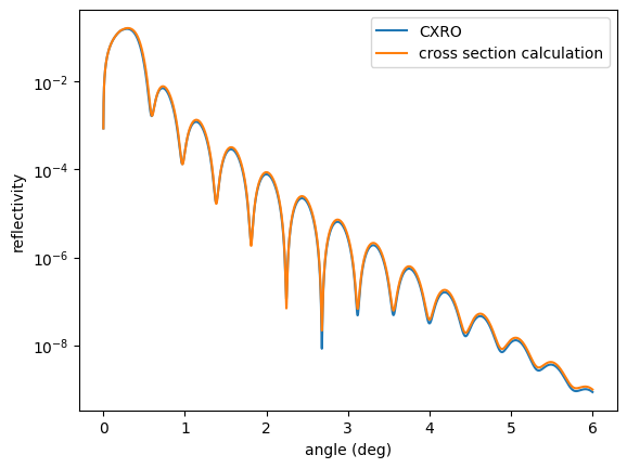
Atomic scattering factors
The calculation of the atomic scattering factors in Nexus can be performed in two different ways. Nexus either calculates Klein-Nishina scattering and uses tabulated values for the photo-electric effect or it uses tabulated values for the real part \(f_1\) and imaginary part \(f_2\) from the Center for X-ray optics [CXRO]. The first version is implemented in CONUSS, the second in GenX, for example. The standard in Nexus is the use of the CXRO values in the range from 1 keV to 30 keV. In the range between 1 eV and 1000 eV always the CXRO values are used, above 30 keV only the cross section calculation is applied.
A problem is that the scattering factors determined in both ways slightly differ, which makes comparison of electronic reflectivities or derived thin film parameters often directly not comparable from different software tools.
Nexus offers global set and get methods to change the calculation method.
With the same definitions for the reflectivity as before one can use
sample.roughness = "a"

plt.semilogy(angles, reflectivity(), label = 'CXRO')

# Set method for the atomic scattering factors
nx.SetAtomicScatteringFactorCXRO(False)

# Get method
print(nx.GetAtomicScatteringFactorCXRO())

plt.semilogy(angles, reflectivity(), label = 'cross section calculation')

plt.legend()
plt.xlabel('angle (deg)')
plt.ylabel('reflectivity')
plt.show()
The code returns a False to indicate the cross section calculation is used instead of the CXRO factors.
The two calculated reflectivities are
This ends the Hello Nexus tutorial.
You can find the jupyter notebooks to the examples here
Notebooks
moessbauer - nb_moessbauer.ipynb.
simple sample - nb_simple_sample.ipynb.
fit - nb_fit.ipynb.
reflectivity - nb_reflectivity.ipynb.
From here, proceed to the tutorials on the specific objects, classes, and methods.