Introduction
Nexus is a flexible and performant package to simulate and fit Moessbauer and nuclear resonant scattering experiments while offering an easy to use Python interface to set up the calculations.
The incoming photon field in the scattering experiment is propagated through all objects in the beam path and the wave field is calculated in response to those objects. Electronic (Klein-Nishina and photoeffect scattering) and nuclear resonant scattering are included. The nuclear transitions are treated fully quantum mechanically in Nexus to obtain the nuclear response function of the object. The wave field is propagated via the transfer-matrix method. Experiments in forward or grazing incidence geometry can be calculated at the moment.
The concept
The basic idea of Nexus is that you set up an Experiment as it was performed.
All elements in the beam path are represented in the software by objects.
An experiment contains a Beam object which holds information on the beam’s polarization and shape.
Objects in the experiment will alter the propagating wave field.
Those objects can be a Sample, an Analyzer or a FixedObject.
For a Sample, the scattering matrices will be calculated by Nexus depending on how the user sets up the sample.
An Analyzer is a photon polarization selective device.
A FixedObject is an object without any energy-dependence, where all scattering factors are provided by the user directly.
The object combinations are arbitrary as long as they are one of those objects.
A more complicated experiment than just a single sample could look like the following
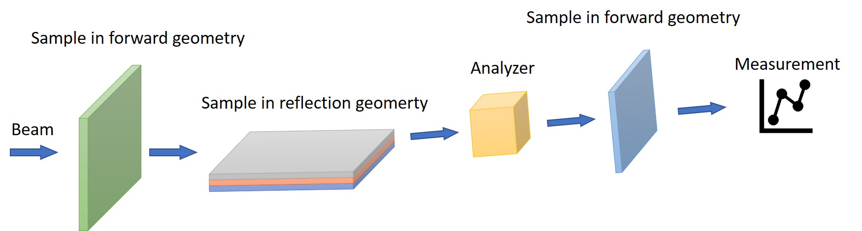
The objects are described by a complex scattering matrix acting on the Beam.
The Beam is propagated through the experiment and a measurement can be calculated.
A Measurement in Nexus is an observable of the experiment.
This is not exactly true because some properties that can be calculated cannot be measured or observed, but let’s not be too strict here.
In this sense, a Measurement can be a measurable quantity, for example, the reflectivity of a thin film system, a Moessbauer spectrum, a time spectrum (the typical notation in the NRS community for a quantum beat).
It can also be a non-observable quantity, like the field intensity profile in a thin film system or the scattering amplitude.
The objects you define in Nexus closely resemble the physical structure.
The Sample consists of \(n\) Layer objects.
A Layer holds information on the geometry and the Material it is made of.
The Material consists of Element objects and stores information on the MoessbauerIsotope and the Hyperfine interactions acting on the MoessbauerIsotope.
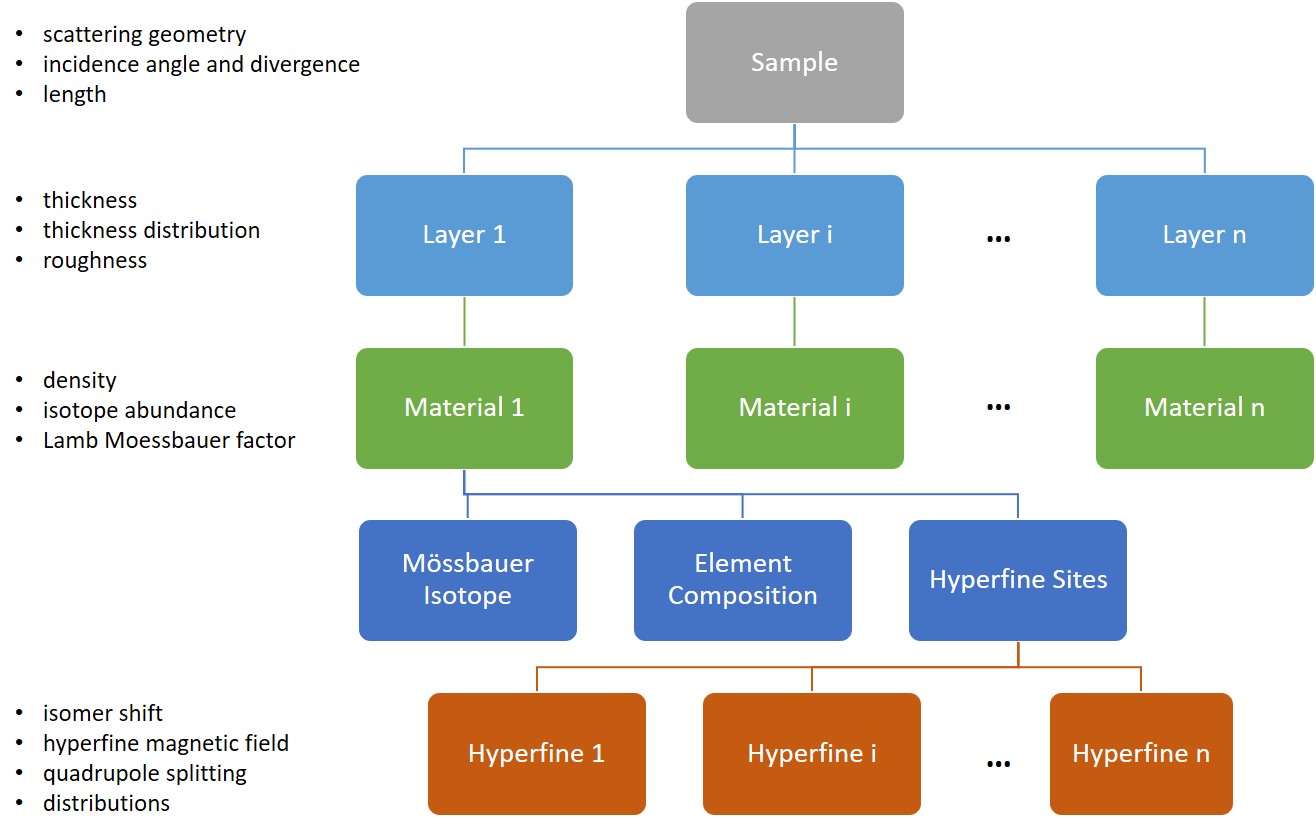
With these building blocks the whole experiment is constructed.
Once the experiment is set up you can define a Measurement type that should be calculated.
For example, calculating a Moessbauer spectrum or a time spectrum of the experiment just differs by applying the MoessbauerSpectrum or TimeSpectrum method to the experiment.
All experimental conditions, like energy or time resolution, are defined in these methods.
Let’s have a look on how objects in Nexus are defined. This is just a basic overview and will give an impression how the Nexus interface works.
# import packages
import nexus as nx
import numpy as np
import matplotlib.pyplot as plt

# you can use any python code in your script

# define nuclear hyperfine parameters
hyperfine_1 = nx.Hyperfine(
    id = "example parameters",   # string id
    isomer = 0.0,                # isomer shift in mm/s
    magnetic_field = 33,         # magnetic field in T
    quadrupole = 0.8,            # quadrupole slitting in mm/s
    isotropic = True,            # 3D distribution in mag and EFG
    # .....)                     # other optional parameters

# define Fe2O3 material
mat_1 = nx.Material(
    id = "my Fe2O3",
    composition = [["Fe", 2],["O", 3]],  # list with element fractions
    density = 5.3,                       # g/cm^3
    isotope = nx.lib.moessbauer.Fe57,    # load isotope from library
    abundance = 0.95,                    # enriched material, "Fe" in composition is made out of 95% of 57-Fe,
    lamb_moessbauer = 0.793,             # Lamb-Moessbauer factor
    hyperfine_sites = [hyperfine_1])     # assign hyperfine parameters

# define a 1000 nm thick layer of Fe2O3
layer_1 = nx.Layer(thickness = 1e3,   # 1000 nm
                   material = mat_1,  # assign material
                   # .....)           # other optional parameters

# define a sample
sample_1 = nx.Sample(layers = [layer_1],  # list with layers in the sample
                     geometry  = "f"      # forward scattering geometry
                     # .....)             # other optional parameters

 # define an unpolarized beam
my_beam = nx.Beam(polarization = 0,
                  # .....)          # other optional parameters

# define an experiment
exp = nx.Experiment(beam = my_beam,                   # input the beam
                    objects = [sample_1],             # put the sample to the object list
                    isotope = nx.lib.moessbauer.Fe57  # set the resonant isotope
                    # .....)                          # other optional parameters

# create a detuning grid for the calculation in mm/s
velocity_grid = np.linspace(-20, 20, 1001)

# define a Measurement, here a Moessbauer spectrum
spectrum = nx.MoessbauerSpectrum(experiment = exp,
                                 velocity = velocity_grid,
                                 # .....)                   # other optional parameters

# calculate the intensity of the spectrum, returns an array of intensities
intensity = spectrum.Calculate()

# plot the result
plt.plot(velocity_grid, intensity)
plt.show()

# post processing
....
Experiments and measurements will be setup step by step. You can use all Nexus objects like any other Python object. However, the object dependencies in Nexus should always be kept in mind, which we will cover in the next section.
Objects in Nexus
Note that all Python class objects can be passed to the next object in any combination the user might think of. Because of Python’s pass by object reference strategy and Nexus internal referencing, this can create complex dependencies. The user should get familiar with Python classes and their attributes because Nexus shows the same behavior.
It is helpful to look at the behavior of the following pure Python code.
class A:
  def __init__(self, input):
    self.variable = input

class B:
  def __init__(self, input):
    self.class_a = input

object_A = A(input = 5)

object_B = B(input = object_A)

print(object_B.class_a.variable)

object_A.variable = 7

print(object_B.class_a.variable)
The two prints will output 5 and 7. Only object_A is changed directly. But as the object_B attribute references to object_A it changes as well.
In Nexus, these class dependencies can be used for flexible fitting of object parameters also with mutual parameter dependencies. Different layers can be made of the same material, than actually every layer holds exactly the same material instance. Changing the material will affect all layers that are made of this material. And this holds for all Nexus objects. Hyperfine sites can be assigned to different materials. Layers can be assigned to different samples. Multilayers can be created with just two layer objects. Fit parameters can be assigned to different objects. Even the same sample can be used in the experiment several times. This might be a little confusing at the beginning but it offers a lot of benefits in combined fitting.
The following examples illustrate this behavior.
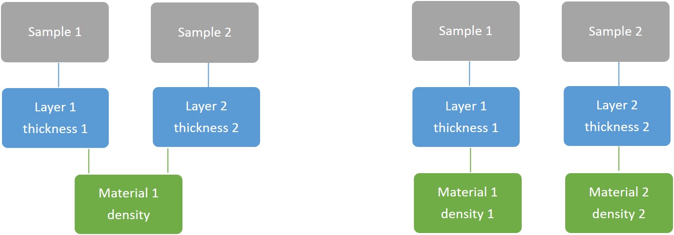
We have created two samples 1 and 2. Each sample consists of one layer, layer 1 and 2, respectively. They might have different thicknesses but be made of the same material. In the left scenario, changing the density of material 1 will affect the layers of both samples. This might be what we want, because we know they are produced in the same way. But we might also want them to be independent because they might be produced in a different manner and the density could be slightly different. In order to do so, we must define two materials, 1 and 2, as shown on the right. Both materials might have the same composition but have different densities 1 and 2. When changing density 1, only layer 1 and sample 1 will be affected.
Note
Use the same object instance only once if you are not sure multiple referencing will affect your Experiment.
Changing object properties even after they have been assigned to another objects will affect the previously initialized object.
Here is an example of the referencing behavior of Nexus.
import nexus as nx

# create a layer from the material library
layer_1 = nx.Layer(thickness = 10,
                   material = nx.Material.Template(nx.lib.material.Fe))

# create two sample with layer_1
# the reference to the layer is passed to the sample
sample_1 = nx.Sample(layers = [layer_1])
sample_2 = nx.Sample(layers = [layer_1])

# change the layer_1 thickness
# and see what happened in the samples
layer_1.thickness = 20

# reference the i-th layer in the sample via sample.layer[i-1]
print(sample_1.layers[0].thickness)
print(sample_2.layers[0].thickness)
# output
Var.value = 20.0, .min = 0.0, .max = inf, .fit: False, .id:
Var.value = 20.0, .min = 0.0, .max = inf, .fit: False, .id:
Both prints show a value of 20.
The object that is printed is not just a float value. Nexus works with a special variable object called Var. This Var will get important when data should be fit. It is a fittable variable which holds information on the fit boundaries and on whether the quantity should be fit or not. Nexus converts your input to a Var automatically. So, no need to care about it if you just want to calculate something.
How Vars will be used for fitting is shown in the next section.
Multi-measurement fitting
Measurements can be fit to experimental data.
However, as has been mentioned, not all measurements are real observables, like the scattering amplitude for example.
Those measurements are not fittable.
One of the big advantages of Nexus is that you can easily fit various Measurements simultaneously with the Fit class.
Those measurements do not need to be from the same experiment and can be completely independent.
Nonetheless, the parameters can depend on the same quantities over several experiments, samples, material, hyperfine sites, and so on.
The image shows a possible dependency tree of various objects that could be fitted.
You can see that the same sample can be used in different experimental conditions and that several measurements of the same experimental setup can enter the Fit class.
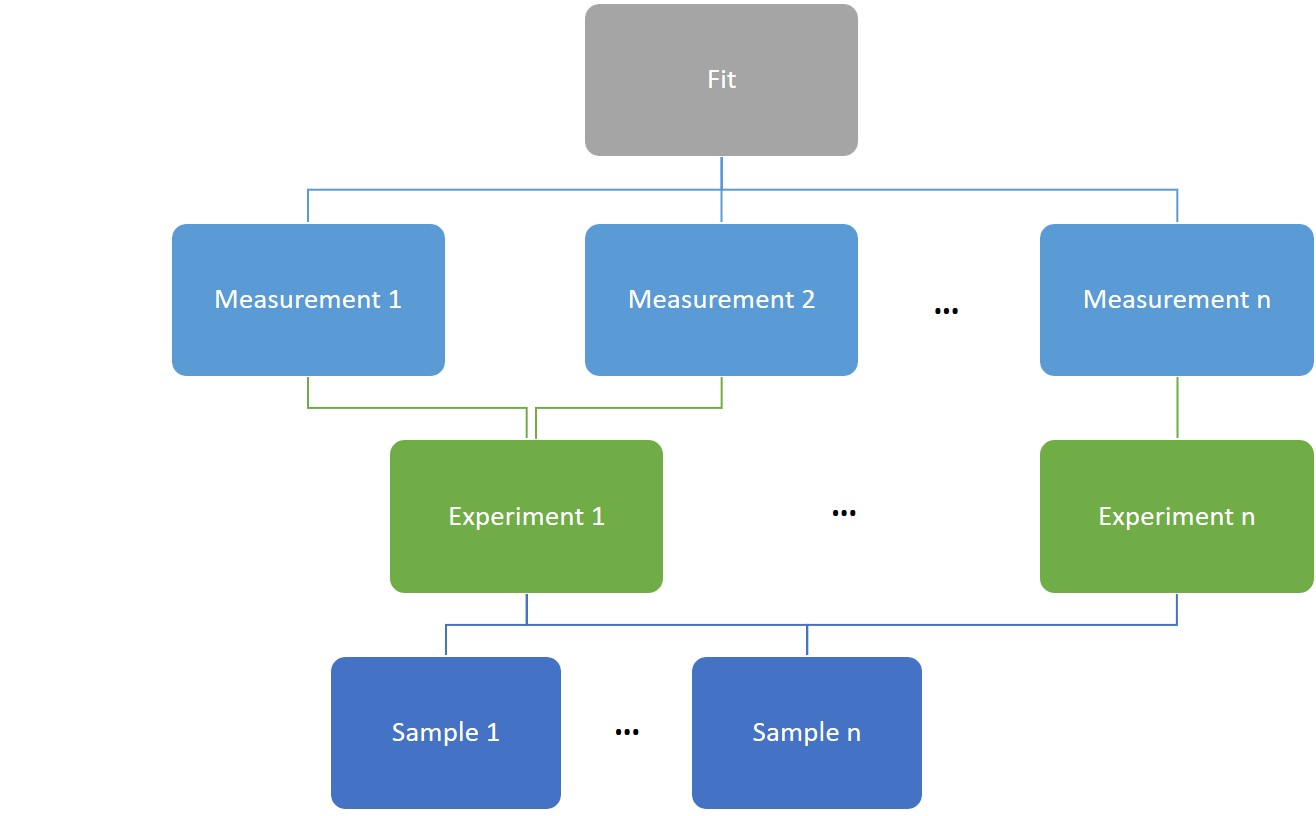
For example, you could have measured a regular reflectivity of a sample at a laboratory diffractometer and use the same sample at an NRS experiment at a beamline where several time spectra and a nuclear reflectivity have been measured. With the fit class you can fit all of those data sets together to get a consistent set of parameters of your sample.
A basic fit example is shown in the following. Here, a Moessbauer spectrum is to be fitted. In the example we only have one fit parameter, the layer thickness, for which we use the Var object directly to make it a fittable parameter.
#assume you have two measured arrays with velocities and intensities
velocity_data = [...]
measured_intensity = [...]

# create an experiment with all needed objects and dependencies
...

# define a layer whose thickness 1000 should be fit in the range of 500 to 2000 nm
# define the parameter as a Var and set the fit attribute to True
layer = nx.Layer(thickness = nx.Var(1000, min = 500, max = 2000, fit = True),
                 material = ...,
                 # .....,  # other optional parameters
                 )

sample = nx.Sample(layers = [layer, ...],
                   # .....,  # other optional parameters
                   )

exp = nx.Experiment(objects = [sample, ...],
                    # .....,  # other optional parameters
                    )

# define a measurement, here a Moessbauer spectrum
# it depends on the layer thickness to be fit
spectrum = nx.MoessbauerSpectrum(experiment = exp,
                                 velocity = velocity_data,
                                 intensitiy_data = measured_intensity
                                 # .....,  # other optional parameters
                                 )

# define a fit object
# it will automatically recognize all Var objects the measurements depend on
fit = nx.Fit(measurements = [spectrum])

# run the fit
fit.Evaluate()

# results will be printed to the command line
This introduction gave a basic overview on what can be done in Nexus. A basic and brief overview on the theory is given in What Nexus calculates. Look at the Installation section on how to get Nexus running on your system. The Tutorial will show you how to use all the methods and give you running examples.