Time dependence
Functions of time
New in version 1.0.4.
Time dependent phenomena are described by a function of time implemented by the FunctionTime class.
The user has to create an instance of this class in Python together with the function definition.
Nexus assumes time values in nanoseconds for the time input of the Function().
The time variable of the Function() must be of type float or int and the return value as well.
class UserTimeDependence(nx.FunctionTime):
    def __init__(self, x0, x1, ...):
        super().__init__("string identifier")
        self.x0 = x0
        self.x1 = x1
        ...

    # times in nanoseconds
    # the time value must be a float or int
    def Function(self, time):
        ...
        y = f(time, x0, x1, ...)
        # the return must be a float or int
        return y
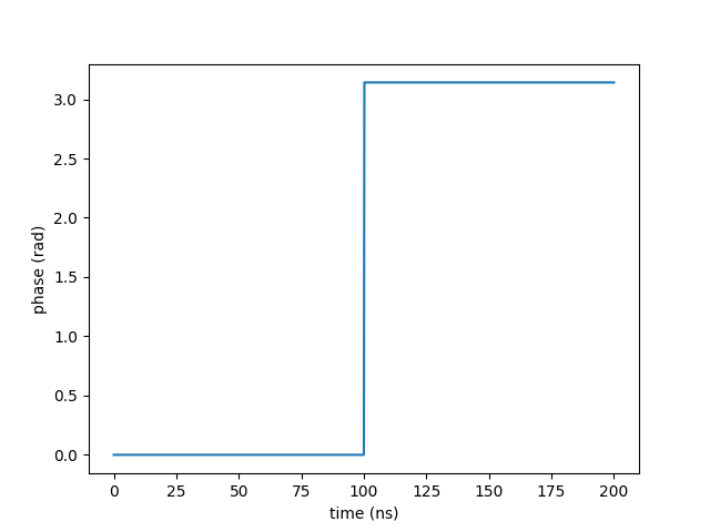
The return value of the function depends in which context the function of time is used. This can be a phase factor for example as used for moving objects. An implementation of a phase jump by \(\pi\) at time \(t_0\) would look this
import nexus as nx
import numpy as np
import matplotlib.pyplot as plt

# define a phase jump function
class PhaseJump(nx.FunctionTime):
    def __init__(self, t0):
        super().__init__("phase jump")
        self.t0 = t0

    def Function(self, time):
        phase = 0
        if time > self.t0:
            phase = np.pi
        return phase

#create a FunctionTime object with a phase jump at 100 ns
func_phase = PhaseJump(100)

# to plot the function
# create a time array in units of nanoseconds
times = np.linspace(0, 200, 1001)

# calculate the phase by calling the function
phase = [func_phase.Function(t) for t in times]

plt.plot(times, phase)
plt.xlabel("time (ns)")
plt.ylabel("phase (rad)")
plt.show()
In order to use fit variables in the FunctionTime object you can pass the Fit objects to the function and register them in the fit_variables attribute.
import nexus as nx
import numpy as np
import matplotlib.pyplot as plt
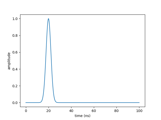
# create a Gaussian pulse
class GaussianPulse(nx.FunctionTime):
def __init__(self, t0, fwhm):
super().__init__("Gaussian pulse")
# create a self. instance of each variable
self.t0 = t0
self.fwhm = fwhm
# register the fit variables in the self.fit_variables
self.fit_variables = [t0, fwhm]
# time in nanoseconds
def Function(self, time):
sigma = self.fwhm.value * 0.424660900144009521361
# catch possible division by zero when fitting
if sigma == 0:
sigma = 1e-299
amp = np.exp(-1/2 * (time - self.t0.value)**2 / sigma**2)
return amp
# create Vars for a Gaussian pulse
t0 = nx.Var(20, min=10, max=30, fit=True, id="t0")
fwhm = nx.Var(5, min=0, max=10, fit=True, id="fwhm")
func_gaussian = GaussianPulse(t0, fwhm)
# print the fit_variables of the function
for elem in list(func_gaussian.fit_variables):
print(elem)
times = np.linspace(0, 100, 1001)
pulse = [func_gaussian.Function(t) for t in times]
plt.plot(times, pulse)
plt.xlabel("time (ns)")
plt.ylabel("amplitude")
plt.show()
to obtain
Var.value = 20.0, .min = 10.0, .max = 30.0, .fit: True, .id: t0
Var.value = 5.0, .min = 1.0, .max = 10.0, .fit: True, .id: fwhm
Special detuning grid
In order to use a time function in Measurement objects that are calculated in the energy domain (via detuning) you need to provide a special detuning grid.
This is needed due special requirements on the Fourier transforms that have to be performed to include the time dependence.
This detuning grid can be generated by the CreateDetuning() method of the FunctionTime class.
It is not assigned to this object, it just returns a valid detuning grid for energy dependent methods.
So, if you have several functions of time you do not need to call the CreateDetuning() method for each function, but only once to create a valid grid and pass it to the methods.
import nexus as nx
import numpy as np
import matplotlib.pyplot as plt

# define a phase jump function
class PhaseJump(nx.FunctionTime):
    def __init__(self, t0):
        super().__init__("phase jump")
        self.t0 = t0

    # time in nanoseconds
    def Function(self, time):
        phase = 0
        if time > self.t0:
            phase = np.pi
        return phase

# initialize the FunctionTime object
func = PhaseJump(20)

# get the special detuning grid needed for calculations in the energy domain
# set the detuing range and the number of points (must be even)
detuning = func.CreateDetuning(400, 2000)

print(detuning)
The detuning grid then is
[-400. -399.6 -399.2 ... 398.8 399.2 399.6]
Moving Sample
A sample motion along the beam propagation direction \(k\) can implemented in all Measurement objects.
The motion should take place on timescales on the order of the nuclear lifetime.
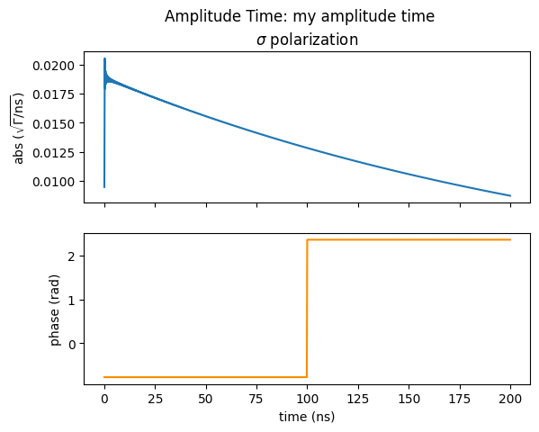
The additional phase factor due to motion is given by \(\varphi(t) = k x(t)\) and the amplitudes \(a(t)\) change to \(a(t) \exp(i \varphi(t)) = a(t) \exp(i k x(t))\).
Here, we calculate the amplitude spectrum of a moving sample in forward direction. We assume the phase jump function created before. Such a motion can be realized with fast piezoelectric materials.
import nexus as nx
import numpy as np
import matplotlib.pyplot as plt

# create function of time
class PhaseJump(nx.FunctionTime):
    def __init__(self, t0):
        super().__init__("phase jump")
        self.t0 = t0

    def Function(self, time):
        phase = 0
        if time > self.t0:
            phase = np.pi
        return phase

# phase jump at 100 ns
func = PhaseJump(100)

# create a proper detuning grid for time dependent calculations
detuning = func.CreateDetuning(400, 4000)

# setup the experiment
mat = nx.Material.Template(nx.lib.material.Fe)

site = nx.Hyperfine(magnetic_field = 0,
                    isotropic = True)

mat.hyperfine_sites = [site]

lay = nx.Layer(id = "iron",
               thickness = 1000,
               material = mat)

sample = nx.Sample(id = "my sample",
                   layers = [lay],
                   geometry = "f",
                   function_time = func) # FunctionTime is applied to the sample

beam = nx.Beam()
beam.LinearSigma()

exp = nx.Experiment(id = "my experiment",
                    beam = beam,
                    objects = [sample],
                    isotope = nx.lib.moessbauer.Fe57)

# create measurement
amp_time = nx.AmplitudeTime(experiment = exp,
                            time_length = 200,
                            time_step = 0.2,
                            id = "my amplitude time",
                            fft_window = "none")

time_axis, amp = amp_time.Calculate()

amp_sigma = amp[:,0]
amp_pi = amp[:,1]

amp_time.Plot(sigma=True, pi=False, polar=True, unwrap=False)
In order to calculate with sample displacements instead of phases you have to scale the displacement by the photon wavevector. The implementation of the phase jump corresponds to a displacement jump by half a wavelength and, for Fe-57, the code will change to
# create function of time
class DisplacementJump(nx.FunctionTime):
    def __init__(self, t0):
        super().__init__("displacement jump")
        self.t0 = t0
        self.k = nx.lib.moessbauer.Fe57.kvector
        self.wavelength = nx.lib.moessbauer.Fe57.wavelength

    def Function(self, time):
        x = 0
        if time > self.t0:
            x = 1/2 * self.wavelength
        phase = self.k * x
        return phase

# phase jump at 100 ns
func = DisplacementJump(100)
Notebooks
amplitude phase jump - nb_amplitude_phase_jump.ipynb.
create detuning - nb_create_detuning.ipynb.